10.1: Induction Motor Transformer Model

The induction machine has two electrically active elements: a rotor and a stator. In normal operation, the stator is excited by alternating voltage. (We consider here only polyphase machines). The stator excitation creates a magnetic field in the form of a rotating, or traveling wave, which induces currents in the circuits of the rotor. Those currents, in turn, interact with the traveling wave to produce torque. To start the analysis of this machine, assume that both the rotor and the stator can be described by balanced, three – phase windings. The two sets are, of course, coupled by mutual inductances which are dependent on rotor position. Stator fluxes are \(\ \left(\lambda_{a}, \lambda_{b}, \lambda_{c}\right)\) and rotor fluxes are \(\ \left(\lambda_{A}, \lambda_{B}, \lambda_{C}\right)\). The flux vs. current relationship is given by:

\(\ \left[\begin{array}{c}
\lambda_{a} \\
\lambda_{b} \\
\lambda_{c} \\
\lambda_{A} \\
\lambda_{B} \\
\lambda_{C}
\end{array}\right]=\left[\begin{array}{ll}
\underline{L}_{S} & \underline{M}_{S R} \\
\underline{M}_{S R}^{T} & \underline{L}_{R}
\end{array}\right]\left[\begin{array}{c}
i_{a} \\
i_{b} \\
i_{c} \\
i_{A} \\
i_{B} \\
i_{C}
\end{array}\right]\label{1}\)

where the component matrices are:

\(\ \underline{\underline{L}}_{S}=\left[\begin{array}{lll}
L_{a} & L_{a b} & L_{a b} \\
L_{a b} & L_{a} & L_{a b} \\
L_{a b} & L_{a b} & L_{a}
\end{array}\right]\label{2}\)

\(\ \underline{\underline{L}}_{R}=\left[\begin{array}{lll}
L_{A} & L_{A B} & L_{A B} \\
L_{A B} & L_{A} & L_{A B} \\
L_{A B} & L_{A B} & L_{A}
\end{array}\right]\label{3}\)

The mutual inductance part of (1) is a circulant matrix:

\(\ \underline{\underline{M}}_{S R}=\left[\begin{array}{lll}
M \cos (p \theta) & M \cos \left(p \theta+\frac{2 \pi}{3}\right) & M \cos \left(p \theta-\frac{2 \pi}{3}\right) \\
M \cos \left(p \theta-\frac{2 \pi}{3}\right) & M \cos (p \theta) & M \cos \left(p \theta+\frac{2 \pi}{3}\right) \\
M \cos \left(p \theta+\frac{2 \pi}{3}\right) & M \cos \left(p \theta-\frac{2 \pi}{3}\right) & M \cos (p \theta)
\end{array}\right]\label{4}\)

To carry the analysis further, it is necessary to make some assumptions regarding operation. To start, assume balanced currents in both the stator and rotor:

\(\ \begin{array}{l}
i_{a}=I_{S} \cos (\omega t) \\
i_{b}=I_{S} \cos \left(\omega t-\frac{2 \pi}{3}\right) \\
i_{c}=I_{S} \cos \left(\omega t+\frac{2 \pi}{3}\right)
\end{array}\label{5}\)

\(\ \begin{aligned}
i_{A} &=I_{R} \cos \left(\omega_{R} t+\xi_{R}\right) \\
i_{B} &=I_{R} \cos \left(\omega_{R} t+\xi_{R}-\frac{2 \pi}{3}\right) \\
i_{C} &=I_{R} \cos \left(\omega_{R} t+\xi_{R}+\frac{2 \pi}{3}\right)
\end{aligned}\label{6}\)

The rotor position \(\ \theta\) can be described by

\(\ \theta=\omega_{m} t+\theta_{0}\label{7}\)

Under these assumptions, we may calculate the form of stator fluxes. As it turns out, we need only write out the expressions for \(\ \lambda_{a}\) and \(\ \lambda_{A}\) to see what is going on:

\(\ \begin{aligned}
\lambda_{a}=&\left(L_{a}-L_{a b}\right) I_{s} \cos (\omega t)+M I_{R}\left(\cos \left(\omega_{R} t+\xi_{R}\right) \cos p\left(\omega_{m}+\theta_{0}\right)\right.\\
&+\cos \left(\omega_{R} t+\xi_{R}+\frac{2 \pi}{3}\right) \cos \left(p\left(\omega_{m} t+\theta_{0}\right)-\frac{2 \pi}{3}\right)+\cos \left(\omega_{R} t+\xi_{R}-\frac{2 \pi}{3}\right) \cos \left(p\left(\omega_{m} t+\theta_{0}\right)+\frac{2 \pi}{3}\right)
\end{aligned}\label{8}\)

which, after reducing some of the trig expressions, becomes:

\(\ \lambda_{a}=\left(L_{a}-L_{a b}\right) I_{s} \cos (\omega t)+\frac{3}{2} M I_{R} \cos \left(\left(p \omega_{m}+\omega_{R}\right) t+\xi_{R}+p \theta_{0}\right)\label{9}\)

Doing the same thing for the rotor phase A yields:

\(\ \begin{aligned}
\lambda_{A}=& M I_{s}\left(\cos p\left(\omega_{m} t+\theta_{0}\right) \cos (\omega t)\right)+\cos \left(p\left(\omega_{m} t+\theta_{0}\right)-\frac{2 \pi}{3}\right) \cos \left(\omega t-\frac{2 \pi}{3}\right) \\
&+\cos \left(p\left(\omega_{m} t+\theta_{0}\right)+\frac{2 \pi}{3}\right) \cos \left(\omega t+\frac{2 \pi}{3}\right)+\left(L_{A}-L_{A B}\right) I_{R} \cos \left(\omega_{R} t+\xi_{R}\right)
\end{aligned}\label{10}\)

This last expression is, after manipulating:

\(\ \lambda_{A}=\frac{3}{2} M I_{s} \cos \left(\left(\omega-p \omega_{m}\right) t-p \theta_{0}\right)+\left(L_{A}-L_{A B}\right) I_{R} \cos \left(\omega_{R} t+\xi_{R}\right)\label{11}\)

These two expressions, 9 and 11 give expressions for fluxes in the armature and rotor windings in terms of currents in the same two windings, assuming that both current distributions are sinusoidal in time and space and represent balanced distributions. The next step is to make another assumption, that the stator and rotor frequencies match through rotor rotation. That is:

\(\ \omega-p \omega_{m}=\omega_{R}\label{12}\)

It is important to keep straight the different frequencies here:

\(\ \omega\) is stator electrical frequency

\(\ \omega_{R}\) is rotor electrical frequency

\(\ \omega_{m}\) is mechanical rotation speed

so that \(\ p \omega_{m}\) is electrical rotation speed.

To refer rotor quantities to the stator frame (i.e. non- rotating), and to work in complex amplitudes, the following definitions are made:

\(\ \lambda_{a}=\operatorname{Re}\left(\underline{\Lambda}_{a} e^{j \omega t}\right)\label{13}\)

\(\ \lambda_{A}=\operatorname{Re}\left(\underline{\Lambda}_{A} e^{j \omega_{R} t}\right)\label{14}\)

\(\ i_{a}=\operatorname{Re}\left(\underline{I}_{a} e^{j \omega t}\right)\label{15}\)

\(\ i_{A}=\operatorname{Re}\left(\underline{I}_{A} e^{j \omega_{R} t}\right)\label{16}\)

With these definitions, the complex amplitudes embodied in 58 and 66 become:

\(\ \underline{\Lambda}_{a}=L_{S} \underline{I}_{a}+\frac{3}{2} M \underline{I}_{A} e^{j\left(\xi_{R}+p \theta_{0}\right)}\label{17}\)

\(\ \underline{\Lambda}_{A}=\frac{3}{2} M \underline{I}_{a} e^{-j p \theta_{0}}+L_{R} \underline{I}_{A} e^{j \xi_{R}}\label{18}\)

There are two phase angles embedded in these expressions: \(\ \theta_{0}\) which describes the rotor physical phase angle with respect to stator current and \(\ \xi_{R}\) which describes phase angle of rotor currents with respect to stator currents. We hereby invent two new rotor variables:

\(\ \left.\underline{\Lambda}_{A R}=\underline{\Lambda}_{A} e^{j p \theta}\right)\label{19}\)

\(\ \underline{I}_{A R}=\underline{I}_{A} e^{j\left(p \theta_{0}+\xi_{R}\right)}\label{20}\)

These are rotor flux and current referred to armature phase angle. Note that \(\ \underline{\Lambda}_{A R}\) and \(\ \underline{I}_{A R}\) have the same phase relationship to each other as do \(\ \underline{\Lambda}_{A}\) and \(\ \underline{I}_{A}\). Using 19 and 20 in 17 and 18, the basic flux/current relationship for the induction machine becomes:

\(\ \left[\begin{array}{l}
\underline{\Lambda}_{a} \\
\underline{\Lambda}_{A R}
\end{array}\right]=\left[\begin{array}{ll}
L_{S} & \frac{3}{2} M \\
\frac{3}{2} M & L_{R}
\end{array}\right]\left[\begin{array}{l}
\underline{I}_{a} \\
\underline{I}_{A R}
\end{array}\right]\label{21}\)

This is an equivalent single- phase statement, describing the flux/current relationship in phase a, assuming balanced operation. The same expression will describe phases b and c.

Voltage at the terminals of the stator and rotor (possibly equivalent) windings is, then:

\(\ \underline{V}_{a}=j \omega \underline{\Lambda}_{a}+R_{a} \underline{I}_{a}\label{22}\)

\(\ \underline{V}_{A R}=j \omega_{R} \underline{\Lambda}_{A R}+R_{A} \underline{I}_{A R}\label{23}\)

or:

\(\ \underline{V}_{a}=j \omega L_{S} \underline{I}_{a}+j \omega \frac{3}{2} M \underline{I}_{A R}+R_{a} \underline{I}_{a}\label{24}\)

\(\ \underline{V}_{A R}=j \omega_{R} \frac{3}{2} M \underline{I}_{a}+j \omega_{R} L_{R} \underline{I}_{A R}+R_{A} \underline{I}_{A R}\label{25}\)

To carry this further, it is necessary to go a little deeper into the machine’s parameters. Note that \(\ L_{S}\) and \(\ L_{R}\) are synchronous inductances for the stator and rotor. These may be separated into space fundamental and “leakage” components as follows:

\(\ L_{S}=L_{a}-L_{a b}=\frac{3}{2} \frac{4}{\pi} \frac{\mu_{0} R l N_{S}^{2} k_{S}^{2}}{p^{2} g}+L_{S l}\label{26}\)

\(\ L_{R}=L_{A}-L_{A B}=\frac{3}{2} \frac{4}{\pi} \frac{\mu_{0} R l N_{R}^{2} k_{R}^{2}}{p^{2} g}+L_{R l}\label{27}\)

Where the normal set of machine parameters holds:

\(\ R\) is rotor radius

\(\ l\) is active length

\(\ g\) is the effective air- gap

\(\ p\) is the number of pole- pairs

\(\ N\) represents number of turns

\(\ k\) represents the winding factor

\(\ S\) as a subscript refers to the stator

\(\ R\) as a subscript refers to the rotor

\(\ L_{l}\) is “leakage” inductance

The two leakage terms \(\ L_{S l}\) and \(\ L_{R l}\) contain higher order harmonic stator and rotor inductances, slot inducances, end- winding inductances and, if necessary, a provision for rotor skew. Essentially, they are used to represent all flux in the rotor and stator that is not mutually coupled.

In the same terms, the stator- to- rotor mutual inductance, which is taken to comprise only a space fundamental term, is:

\(\ M=\frac{4}{\pi} \frac{\mu_{0} R l N_{S} N_{R} k_{S} k_{R}}{p^{2} g}\label{28}\)

Note that there are, of course, space harmonic mutual flux linkages. If they were to be included, they would hair up the analysis substantially. We ignore them here and note that they do have an effect on machine behavior, but that effect is second- order.

Air- gap permeance is defined as:

\(\ \wp_{a g}=\frac{4}{\pi} \frac{\mu_{0} R l}{p^{2} g}\label{29}\)

so that the inductances are:

\(\ L_{S}=\frac{3}{2} \wp_{a g} k_{S}^{2} N_{S}^{2}+L_{S l}\label{30}\)

\(\ L_{R}=\frac{3}{2} \wp_{a g} k_{R}^{2} N_{R}^{2}+L_{R l}\label{31}\)

\(\ M=\wp_{a g} N_{S} N_{R} k_{S} k_{R}\label{32}\)

Here we define “slip” s by:

\(\ \omega_{R}=s \omega\label{33}\)

so that

\(\ s=1-\frac{p \omega_{m}}{\omega}\label{34}\)

Then the voltage balance equations become:

\(\ \underline{V}_{a}=j \omega\left(\frac{3}{2} \wp_{a g} k_{S}^{2} N_{S}^{2}+L_{S l}\right) \underline{I}_{a}+j \omega \frac{3}{2} \wp_{a g} N_{S} N_{R} k_{S} k_{R} \underline{I}_{A R}+R_{a} \underline{I}_{a}\label{35}\)

\(\ \underline{V}_{A R}=j s \omega \frac{3}{2} \wp_{a g} N_{S} N_{R} k_{S} k_{R} \underline{I}_{a}+j s \omega\left(\frac{3}{2} \wp_{a g} k_{R}^{2} N_{R}^{2}+L_{R l}\right) \underline{I}_{A R}+R_{A} \underline{I}_{A R}\label{36}\)

At this point, we are ready to define rotor current referred to the stator. This is done by assuming an effective turns ratio which, in turn, defines an equivalent stator current to produce the same fundamental MMF as a given rotor current:

\(\ \underline{I}_{2}=\frac{N_{R} k_{R}}{N_{S} k_{S}} \underline{I}_{A R}\label{37}\)

Now, if we assume that the rotor of the machine is shorted so that V AR = 0 and do some manipulation we obtain:

\(\ \underline{V}_{a}=j\left(X_{M}+X_{1}\right) \underline{I}_{a}+j X_{M} \underline{I}_{2}+R_{a} \underline{I}_{a}\label{38}\)

\(\ 0=j X_{M} \underline{I}_{a}+j\left(X_{M}+X_{2}\right) \underline{I}_{2}+\frac{R_{2}}{s} \underline{I}_{2}\label{39}\)

where the following definitions have been made:

\(\ X_{M}=\frac{3}{2} \omega \wp_{a g} N_{S}^{2} k_{S}^{2}\label{40}\)

\(\ X_{1}=\omega L_{S l}\label{41}\)

\(\ X_{2}=\omega L_{R l}\left(\frac{N_{S} k_{S}}{N_{R} k_{R}}\right)^{2}\label{42}\)

\(\ R_{2}=R_{A}\left(\frac{N_{S} k_{S}}{N_{R} k_{R}}\right)^{2}\label{43}\)

These expressions describe a simple equivalent circuit for the induction motorshow in Figure 2. We will amplify on this equivalent circuit anon.

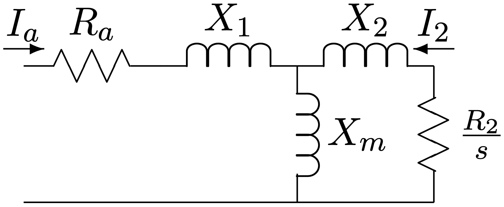Figure 2: Equivalent Circuit

Effective Air-Gap: Carter’s Coefficient

In induction motors, where the air-gap is usually quite small, it is necessary to correct the air-gap permeance for the effect of slot openings. These make the permeance of the air-gap slightly smaller than calculated from the physical gap, effectively making the gap a bit bigger. The ratio of effective to physical gap is:

\(\ g_{\mathrm{eff}}=g \frac{t+s}{t+s-g f(\alpha)}\label{44}\)

where

\(\ f(\alpha)=f\left(\frac{s}{2 g}\right)=\alpha \tan (\alpha)-\log \sec \alpha\label{45}\)