10.3: Squirrel Cage Machine Model

Now we derive a circuit model for the squirrel-cage motor using field analytical techniques. The model consists of two major parts. The first of these is a description of stator flux in terms of stator and rotor currents. The second is a description of rotor current in terms of air- gap flux. The result of all of this is a set of expressions for the elements of the circuit model for the induction machine.

To start, assume that the rotor is symmetrical enough to carry a surface current, the fundamental of which is:

\(\ \begin{aligned}
\bar{K}_{r} &=\bar{\imath}_{z} \operatorname{Re}\left(\underline{K}_{r} e^{j\left(s \omega t-p \phi^{\prime}\right)}\right) \\
&=\bar{\imath}_{z} \operatorname{Re}\left(\underline{K}_{r} e^{j(\omega t-p \phi)}\right)
\end{aligned}\label{58}\)

Note that in 58 we have made use of the simple transformation between rotor and stator coordinates:

\(\ \phi^{\prime}=\phi-\omega_{m} t\label{59}\)

and that

\(\ p \omega_{m}=\omega-\omega_{r}=\omega(1-s)\label{60}\)

Here, we have used the following symbols:

\(\ \underline{K}_{r}\)	is complex amplitude of rotor surface current
\(\ \mathcal{S}\)	is per- unit “slip”
\(\ \omega\)	is stator electrical frequency
\(\ \omega_{r}\)	is rotor electrical frequency
\(\ \omega_{m}\)	is rotational speed

The rotor current will produce an air- gap flux density of the form:

\(\ B_{r}=R e\left(\underline{B}_{r} e^{j(\omega t-p \phi)}\right)\label{61}\)

where

\(\ \underline{B}_{r}=-j \mu_{0} \frac{R}{p g} \underline{K}_{r}\label{62}\)

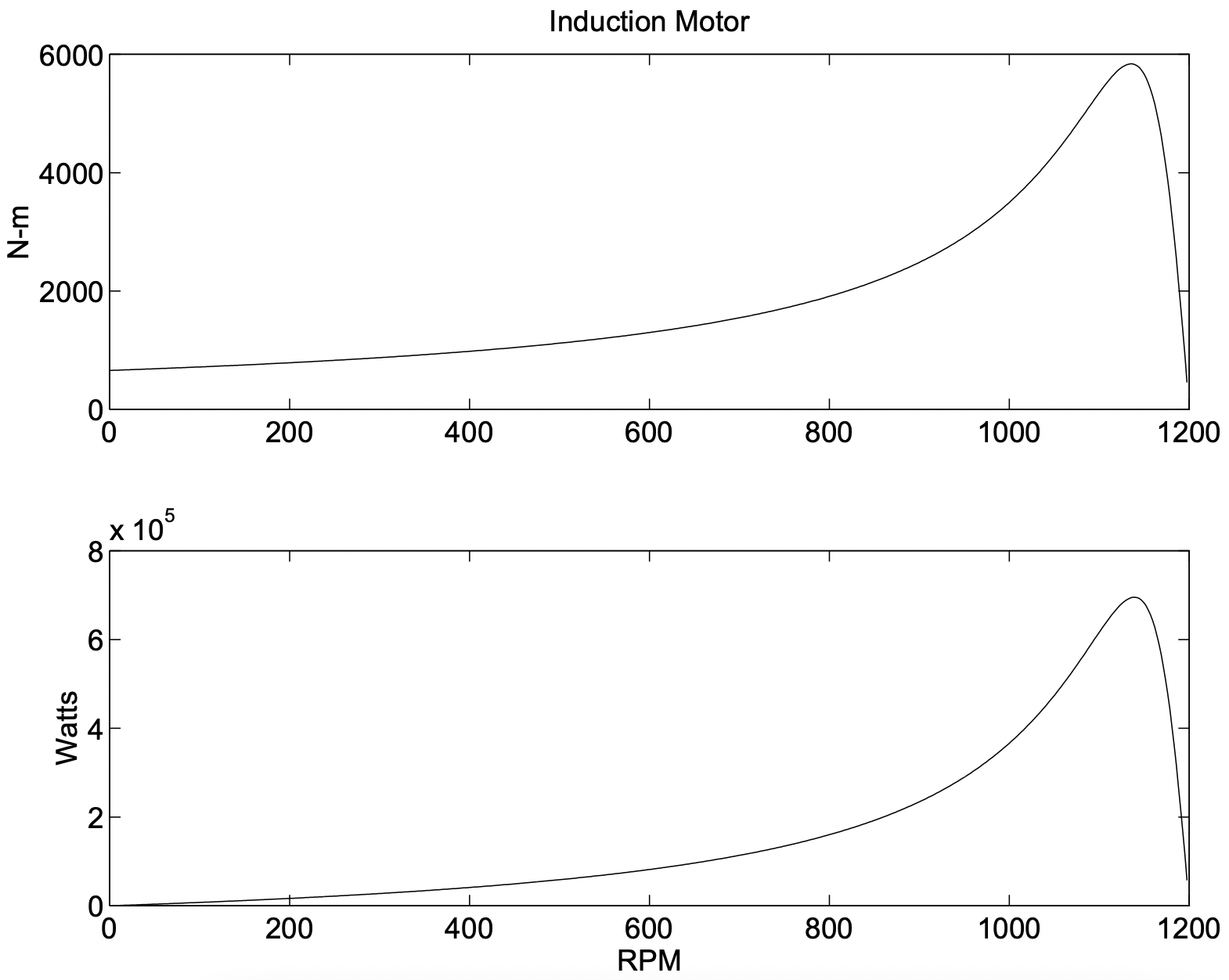Figure 3: Torque and Power vs. Speed for Example Motor

Note that this describes only radial magnetic flux density produced by the space fundamental of rotor current. Flux linked by the armature winding due to this flux density is:

\(\ \lambda_{A R}=l N_{S} k_{S} \int_{-\frac{\pi}{p}}^{0} B_{r}(\phi) R d \phi\label{63}\)

This yields a complex amplitude for \(\ \lambda_{A R}\):

\(\ \lambda_{A R}=\operatorname{Re}\left(\underline{\Lambda}_{A R} e^{j \omega t}\right)\label{64}\)

where

\(\ \underline{\Lambda}_{A R}=\frac{2 l \mu_{0} R^{2} N_{S} k_{S}}{p^{2} g} \underline{K}_{r}\label{65}\)

Adding this to flux produced by the stator currents, we have an expression for total stator flux:

\(\ \underline{\Lambda}_{a}=\left(\frac{3}{2} \frac{4}{\pi} \frac{\mu_{0} N_{S}^{2} R l k_{S}^{2}}{p^{2} g}+L_{S l}\right) \underline{I}_{a}+\frac{2 l \mu_{0} R^{2} N_{S} k_{S}}{p^{2} g} \underline{K}_{r}\label{66}\)

Expression 66 motivates a definiton of an equivalent rotor current I2 in terms of the space fundamental of rotor surface current density:

\(\ \underline{I}_{2}=\frac{\pi}{3} \frac{R}{N_{S} k_{S}} \underline{K}_{z}\label{67}\)

Then we have the simple expression for stator flux:

\(\ \underline{\Lambda}_{a}=\left(L_{a d}+L_{S l}\right) \underline{I}_{a}+L_{a d} \underline{I}_{2}\label{68}\)

where \(\ L_{a d}\) is the fundamental space harmonic component of stator inductance:

\(\ L_{a d}=\frac{3}{2} \frac{4}{\pi} \frac{\mu_{0} N_{S}^{2} k_{S}^{2} R l}{p^{2} g}\label{69}\)

The second part of this derivation is the equivalent of finding a relationship between rotor flux and \(\ I_{2}\). However, since this machine has no discrete windings, we must focus on the individual rotor bars.

Assume that there are \(\ N_{R}\) slots in the rotor. Each of these slots is carrying some current. If the machine is symmetrical and operating with balanced currents, we may write an expression for current in the \(\ k^{t h}\) slot as:

\(\ i_{k}=\operatorname{Re}\left(\underline{I}_{k} e^{j s \omega t}\right)\label{70}\)

where

\(\ \underline{I}_{k}=\underline{I} e^{-j \frac{2 \pi p}{N_{R}}}\label{71}\)

and \(\ \underline{I}\) is the complex amplitude of current in slot number zero. Expression 71 shows a uniform progression of rotor current phase about the rotor. All rotor slots carry the same current, but that current is phase retarded (delayed) from slot to slot because of relative rotation of the current wave at slip frequency.

The rotor current density can then be expressed as a sum of impulses:

\(\ K_{z}=R e\left(\sum_{k=0}^{N_{R}-1} \frac{1}{R} \underline{I} e^{j\left(\omega_{r} t-k \frac{2 \pi p}{N_{R}}\right)} \delta\left(\phi^{\prime}-\frac{2 \pi k}{N_{R}}\right)\right)\label{72}\)

The unit impulse function \(\ \delta()\) is our way of approximating the rotor current as a series of impulsive currents around the rotor.

This rotor surface current may be expressed as a fourier series of traveling waves:

\(\ K_{z}=\operatorname{Re}\left(\sum_{n=-\infty}^{\infty} \underline{K}_{n} e^{j\left(\omega_{r} t-n p \phi^{\prime}\right)}\right)\label{73}\)

Note that in 73, we are allowing for negative values of the space harmonic index \(\ n\) to allow for reverse- rotating waves. This is really part of an expansion in both time and space, although we are considering only the time fundamental part. We may recover the \(\ n^{t h}\) space harmonic component of 73 by employing the following formula:

\(\ \underline{K}_{n}=<\frac{1}{\pi} \int_{0}^{2 \pi} K_{r}(\phi, t) e^{-j\left(\omega_{r} t-n p \phi\right)} d \phi>\label{74}\)

Here the brackets <> denote time average and are here beause of the two- dimensional nature of the expansion. To carry out 74 on 72, first expand 72 into its complex conjugate parts:

\(\ K_{r}=\frac{1}{2} \sum_{k=0}^{N_{R}-1}\left\{\frac{\underline{I}}{R} e^{j\left(\omega_{r} t-k \frac{2 \pi p}{N_{R}}\right)}+\frac{\underline{I}^{*}}{R} e^{-j\left(\omega_{r} t-k \frac{2 \pi p}{N_{R}}\right)}\right\} \delta\left(\phi^{\prime}-\frac{2 \pi k}{N_{R}}\right)\label{75}\)

If 75 is used in 74, the second half of 75 results in a sum of terms which time average to zero. The first half of the expression results in:

\(\ \underline{K}_{n}=\frac{I}{2 \pi R} \int_{0}^{2 \pi} \sum_{k=0}^{N_{R}-1} e^{-j \frac{2 \pi p k}{N_{R}}} e^{j n p \phi} \delta\left(\phi-\frac{2 \pi k}{N_{R}}\right) d \phi\label{76}\)

The impulse function turns the integral into an evaluation of the rest of the integrand at the impulse. What remains is the sum:

\(\ \underline{K}_{n}=\frac{\underline{I}}{2 \pi R} \sum_{k=0}^{N_{R}-1} e^{j(n-1) \frac{2 \pi k p}{N_{R}}}\label{77}\)

The sum in 77 is easily evaluated. It is:

\(\ \sum_{k=0}^{N_{R}-1} e^{j \frac{2 \pi k p(n-1)}{N_{R}}}=\left\{\begin{array}{ll}
N_{R} & \text { if }(n-1) \frac{P}{N_{R}}=\text { integer } \\
0 & \text { otherwise }
\end{array}\right.\label{78}\)

The integer in 78 may be positive, negative or zero. As it turns out, only the first three of these (zero, plus and minus one) are important, because these produce the largest magnetic fields and therefore fluxes. These are:

\(\ \begin{aligned}
(n-1) \frac{p}{N_{R}}=-1 & \text { or } n=-\frac{N_{R}-p}{p} \\
=0 \quad & \text { or } n=1 \\
=1 \quad & \text { or } n=\frac{N_{R}+p}{p}
\end{aligned}\label{79}\)

Note that 79 appears to produce space harmonic orders that may be of non- integer order. This is not really true: is is necessary that \(\ np\) be an integer, and 79 will always satisfy that condition.

So, the harmonic orders of interest to us are one and

\(\ n_{+}=\frac{N_{R}}{p}+1\label{80}\)

\(\ n_{-}=-\left(\frac{N_{R}}{p}-1\right)\label{81}\)

Each of the space harmonics of the squirrel- cage current will produce radial flux density. A surface current of the form:

\(\ K_{n}=R e\left(\frac{N_{R} \underline{I}}{2 \pi R} e^{j\left(\omega_{r} t-n p \phi^{\prime}\right)}\right)\label{82}\)

produces radial magnetic flux density:

\(\ B_{r n}=\operatorname{Re}\left(\underline{B}_{r n} e^{j\left(\omega_{r} t-n p \phi^{\prime}\right)}\right)\label{83}\)

where

\(\ \underline{B}_{r n}=-j \frac{\mu_{0} N_{R} \underline{I}}{2 \pi n p g}\label{84}\)

In turn, each of the components of radial flux density will produce a component of induced voltage. To calculate that, we must invoke Faraday’s law:

\(\ \nabla \times \bar{E}=-\frac{\partial \bar{B}}{\partial t}\label{85}\)

The radial component of 85, assuming that the fields do not vary with \(\ Z\), is:

\(\ \frac{1}{R} \frac{\partial}{\partial \phi} E_{z}=-\frac{\partial B_{r}}{\partial t}\label{86}\)

Or, assuming an electric field component of the form:

\(\ E_{z n}=\operatorname{Re}\left(\underline{E}_{n} e^{j\left(\omega_{r} t-n p \phi\right)}\right)\label{87}\)

Using 84 and 87 in 86, we obtain an expression for electric field induced by components of airgap flux:

\(\ \underline{E}_{n}=\frac{\omega_{r} R}{n p} \underline{B}_{n}\label{88}\)

\(\ \underline{E}_{n}=-j \frac{\mu_{0} N_{R} \omega_{r} R}{2 \pi g(n p)^{2}} \underline{I}\label{89}\)

Now, the total voltage induced in a slot pushes current through the conductors in that slot. We may express this by:

\(\ \underline{E}_{1}+\underline{E}_{n-}+\underline{E}_{n+}=\underline{Z}_{s l o t} \underline{I}\label{90}\)

Now: in 90, there are three components of air- gap field. \(\ E_{1}\) is the space fundamental field, produced by the space fundamental of rotor current as well as by the space fundamental of stator current. The other two components on the left of 90 are produced only by rotor currents and actually represent additional reactive impedance to the rotor. This is often called zigzag leakage inductance. The parameter Zslot represents impedance of the slot itself: resistance and reactance associated with cross- slot magnetic fields. Then 90 can be re-written as:

\(\ \underline{E}_{1}=\underline{Z}_{s l o t} \underline{I}+j \frac{\mu_{0} N_{R} \omega_{r} R}{2 \pi g}\left(\frac{1}{\left(n_{+} p\right)^{2}}+\frac{1}{\left(n_{-} p\right)^{2}}\right) \underline{I}\label{91}\)

To finish this model, it is necessary to translate 91 back to the stator. See that 67 and 77 make the link between \(\ \underline{I}\) and \(\ \underline{I}_{2}\):

\(\ \underline{I}_{2}=\frac{N_{R}}{6 N_{S} k_{S}} \underline{I}\label{92}\)

Then the electric field at the surface of the rotor is:

\(\ \underline{E}_{1}=\left[\frac{6 N_{S} k_{S}}{N_{R}} \underline{Z}_{s l o t}+j \omega_{r} \frac{3}{\pi} \frac{\mu_{0} N_{S} k_{S} R}{g}\left(\frac{1}{\left(n_{+} p\right)^{2}}+\frac{1}{\left(n_{-} p\right)^{2}}\right)\right] \underline{I}_{2}\label{93}\)

This must be translated into an equivalent stator voltage. To do so, we use 88 to translate 93 into a statement of radial magnetic field, then find the flux liked and hence stator voltage from that. Magnetic flux density is:

\(\ \begin{aligned}
\underline{B}_{r} &=\frac{p \underline{E}_{1}}{\omega_{r} R} \\
&=\left[\frac{6 N_{S} k_{S} p}{N_{R} R}\left(\frac{R_{s l o t}}{\omega_{r}}+j L_{s l o t}\right)+j \frac{3}{\pi} \frac{\mu_{0} N_{S} k_{S} p}{g}\left(\frac{1}{\left(n_{+} p\right)^{2}}+\frac{1}{\left(n_{-} p\right)^{2}}\right)\right] \underline{I}_{2}
\end{aligned}\label{94}\)

where the slot impedance has been expressed by its real and imaginary parts:

\[\ \underline{Z}_{s l o t}=R_{s l o t}+j \omega_{r} L_{s l o t}\label{95} \]

Flux linking the armature winding is:

\[\ \lambda_{a g}=N_{S} k_{S} l R \int_{-\frac{\pi}{2 p}}^{0} \operatorname{Re}\left(\underline{B}_{r} e^{j(\omega t-p \phi)}\right) d \phi\label{96} \]

Which becomes:

\[\ \lambda_{a g}=\operatorname{Re}\left(\underline{\Lambda}_{a g} e^{j \omega t}\right)\label{97} \]

where:

\[\ \underline{\Lambda}_{a g}=j \frac{2 N_{S} k_{S} l R}{p} \underline{B}_{r}\label{98} \]

Then “air- gap” voltage is:

\[\ \begin{aligned}
\underline{V}_{a g} &=j \omega \underline{\Lambda}_{a g}=-\frac{2 \omega N_{S} k_{S} l R}{p} \underline{B}_{r} \\
&=-\underline{I}_{2}\left[\frac{12 l N_{S}^{2} k_{S}^{2}}{N_{R}}\left(j \omega L_{s l o t}+\frac{R_{2}}{s}\right)+j \omega \frac{6}{\pi} \frac{\mu_{0} R l N_{S}^{2} k_{S}^{2}}{g}\left(\frac{1}{\left(n_{+} p\right)^{2}}+\frac{1}{\left(n_{-} p\right)^{2}}\right)\right]
\end{aligned}\label{99} \]

Expression 99 describes the relationship between the space fundamental air- gap voltage \(\ \underline{V}_{a g}\) and rotor current \(\ \underline{I}_{2}\). This expression fits the equivalent circuit of Figure 4 if the definitions made below hold:

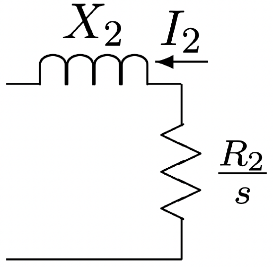Figure 4: Rotor Equivalent Circuit

\[\ X_{2}=\omega \frac{12 l N_{S}^{2} k_{S}^{2}}{N_{R}} L_{\mathrm{slot}}+\omega \frac{6}{\pi} \frac{\mu_{0} R l N_{S}^{2} k_{S}^{2}}{g}\left(\frac{1}{\left(N_{R}+p\right)^{2}}+\frac{1}{\left(N_{R}-p\right)^{2}}\right)\label{100} \]

\[\ R_{2}=\frac{12 l N_{S}^{2} k_{S}^{2}}{N_{R}} R_{\text {slot }}\label{101} \]

The first term in 100 expresses slot leakage inductance for the rotor. Similarly, 101 expresses rotor resistance in terms of slot resistance. Note that Lslot and Rslot are both expressed per unit length. The second term in 100 expresses the “zigzag” leakage inductance resulting from harmonics on the order of rotor slot pitch.

Next, see that armature flux is just equal to air- gap flux plus armature leakage inductance. That is, 68 could be written as:

\[\ \underline{\Lambda}_{a}=\underline{\Lambda}_{a g}+L_{a l} \underline{I}_{a}\label{102} \]

There are a number of components of stator slot leakage \(\ L_{a l}\), each representing flux paths that do not directly involve the rotor. Each of the components adds to the leakage inductance. The most prominent components of stator leakage are referred to as slot, belt, zigzag, end winding, and skew. Each of these will be discussed in the following paragraphs.

Belt and zigzag leakage components are due to air- gap space harmonics. As it turns out, these are relatively complicated to estimate, but we may get some notion from our first- order view of the machine. The trouble with estimating these leakage components is that they are not really independent of the rotor, even though we call them “leakage”. Belt harmonics are of order \(\ n=5\) and \(\ n=7\). If there were no rotor coupling, the belt harmonic leakage terms would be:

\[\ X_{a g 5}=\frac{3}{2} \frac{4}{\pi} \frac{\mu_{0} N_{S}^{2} k_{5}^{2} R l}{5^{2} p^{2} g}\label{103} \]

\[\ X_{a g 7}=\frac{3}{2} \frac{4}{\pi} \frac{\mu_{0} N_{S}^{2} k_{7}^{2} R l}{7^{2} p^{2} g}\label{104} \]

The belt harmonics link to the rotor, however, and actually appear to be in parallel with components of rotor impedance appropriate to 5p and 7p pole- pair machines. At these harmonic orders we can usually ignore rotor resistance so that rotor impedance is purely inductive. Those components are:

\[\ X_{2,5}=\omega \frac{12 l N_{S}^{2} k_{5}^{2}}{N_{R}} L_{\mathrm{slot}}+\omega \frac{6}{\pi} \frac{\mu_{0} R l N_{S}^{2} k_{5}^{2}}{g}\left(\frac{1}{\left(N_{R}+5 p\right)^{2}}+\frac{1}{\left(N_{R}-5 p\right)^{2}}\right)\label{105} \]

\[\ X_{2,7}=\omega \frac{12 l N_{S}^{2} k_{7}^{2}}{N_{R}} L_{\mathrm{slot}}+\omega \frac{6}{\pi} \frac{\mu_{0} R l N_{S}^{2} k_{7}^{2}}{g}\left(\frac{1}{\left(N_{R}+7 p\right)^{2}}+\frac{1}{\left(N_{R}-7 p\right)^{2}}\right)\label{106} \]

In the simple model of the squirrel cage machine, because the rotor resistances are relatively small and slip high, the effect of rotor resistance is usually ignored. Then the fifth and seventh harmonic components of belt leakage are:

\[\ X_{5}=X_{a g 5} \| X_{2,5}\label{107} \]

\[\ X_{7}=X_{a g 7} \| X_{2,7}\label{108} \]

Stator zigzag leakage is from those harmonics of the orders \(\ p n_{s}=N_{s l o t s} \pm p\) where \(\ N_{\text {slots }}\).

\[\ X_{z}=\frac{3}{2} \frac{4}{\pi} \frac{\mu_{0} N_{S}^{2} R l}{g}\left(\frac{k_{n_{s}+}}{\left(N_{\text {slots }}+p\right)^{2}}+\frac{k_{n_{s}-}}{\left(N_{\text {slots }}-p\right)^{2}}\right)\label{109} \]

Note that these harmonic orders do not tend to be shorted out by the rotor cage and so no direct interaction with the cage is ordinarily accounted for.

In order to reduce saliency effects that occur because the rotor teeth will tend to try to align with the stator teeth, induction motor designers always use a different number of slots in the rotor and stator. There still may be some tendency to align, and this produces “cogging” torques which in turn produce vibration and noise and, in severe cases, can retard or even prevent starting. To reduce this tendency to “cog”, rotors are often built with a little “skew”, or twist of the slots from one end to the other. Thus, when one tooth is aligned at one end of the machine, it is un-aligned at the other end. A side effect of this is to reduce the stator and rotor coupling by just a little, and this produces leakage reactance. This is fairly easy to estimate. Consider, for example, a space-fundamental flux density \(\ B_{r}=B_{1} \cos p \theta\), linking a (possibly) skewed full-pitch current path:

\(\ \lambda=\int_{-\frac{l}{2}}^{\frac{l}{2}} \int_{-\frac{\pi}{2 p}+\frac{\varsigma}{p} \frac{x}{l}}^{\frac{\pi}{2 p}+\frac{\varsigma}{p} \frac{x}{l}} B_{1} \cos p \theta R d \theta d x\)

Here, the skew in the rotor is \(\ \varsigma\) electrical radians from one end of the machine to the other. Evaluation of this yields:

\(\ \lambda=\frac{2 B_{1} R l}{p} \frac{\sin \frac{\varsigma}{2}}{\frac{\varsigma}{2}}\)

Now, the difference between what would have been linked by a non-skewed rotor and what is linked by the skewed rotor is the skew leakage flux, now expressible as:

\(\ X_{k}=X_{a g}\left(1-\frac{\sin \frac{\varsigma}{2}}{\frac{\varsigma}{2}}\right)\)

The final component of leakage reactance is due to the end windings. This is perhaps the most difficult of the machine parameters to estimate, being essentially three-dimensional in nature. There are a number of ways of estimating this parameter, but for our purposes we will use a simplified parameter from AlgerEquation \ref{1}:

\(\ X_{e}=\frac{14}{4 \pi^{2}} \frac{q}{2} \frac{\mu_{0} R N_{a}^{2}}{p^{2}}(p-0.3)\)

As with all such formulae, extreme care is required here, since we can give little guidance as to when this expression is correct or even close. And we will admit that a more complete treatment of this element of machine parameter construction would be an improvement.

Harmonic Order Rotor Resistance and Stray Load Losses

It is important to recognize that the machine rotor “sees” each of the stator harmonics in essentially the same way, and it is quite straightforward to estimate rotor parameters for the harmonic orders, as we have done just above. Now, particularly for the “belt” harmonic orders, there are rotor currents flowing in response to stator mmf’s at fifth and seventh space harmonic order. The resistances attributable to these harmonic orders are:

\[\ R_{2,5}=\frac{12 l N_{s}^{2} k_{5}^{2}}{N_{R}} R_{\operatorname{slot}, 5}\label{110} \]

\[\ R_{2,7}=\frac{12 l N_{s}^{2} k_{7}^{2}}{N_{R}} R_{\mathrm{slot}, 7}\label{111} \]

The higher-order slot harmonics will have relative frequencies (slips) that are:

\[\ s_{n}=1 \mp(1-s) n\left\{\begin{array}{l}
n=6 k+1 \\
n=6 k-1
\end{array}\right\} \mathrm{k} \text { an integer }\label{112} \]

The induction motor electromagnetic interaction can now be described by an augmented magnetic circuit as shown in Figure 17. Note that the terminal flux of the machine is the sum of all of the harmonic fluxes, and each space harmonic is excited by the same current so the individual harmonic components are in series.

Each of the space harmonics will have an electromagnetic interaction similar to the fundamental: power transferred across the air-gap is:

\(\ P_{e m, n}=3 I_{2, n}^{2} \frac{R_{2, n}}{s_{n}}\)

Of course dissipation in each circuit is:

\(\ P_{d, n}=3 I_{2, n}^{2} R_{2, n}\)

leaving

\(\ P_{m, n}=3 I_{2, n}^{2} \frac{R_{2, n}}{s_{n}}\left(1-s_{n}\right)\)

Note that this equivalent circuit has provision for two sets of circuits which look like “cages”. In fact one of these sets is for the solid rotor body if that exists. We will discuss that anon. There is also a provision \(\ \left(r_{c}\right)\) for loss in the stator core iron.

Power deposited in the rotor harmonic resistance elements is characterized as “stray load” loss because it is not easily computed from the simple machine equivalent circuit.

Slot Models

Some of the more interesting things that can be done with induction motors have to do with the shaping of rotor slots to achieve particular frequency-dependent effects. We will consider here three cases, but there are many other possibilities.

First, suppose the rotor slots are representable as being rectangular, as shown in Figure 5, and assume that the slot dimensions are such that diffusion effects are not important so that current in the slot conductor is approximately uniform. In that case, the slot resistance and inductance per unit length are:

\[\ R_{\mathrm{slot}}=\frac{1}{w_{s} h_{s} \sigma}\label{113} \]

\[\ L_{\mathrm{slot}}=\mu_{0} \frac{h_{s}}{3 w_{s}}\label{114} \]

The slot resistance is obvious, the slot inductance may be estimated by recognizing that if the current in the slot is uniform, magnetic field crossing the slot must be:

\(\ H_{y}=\frac{I}{w_{s}} \frac{x}{h_{s}}\)

Then energy stored in the field in the slot is simply:

\(\ \frac{1}{2} L_{\mathrm{slot}} I^{2}=w_{s} \int_{0}^{h_{s}} \frac{\mu_{0}}{2}\left(\frac{I x}{w_{s} h_{s}}\right)^{2} d x=\frac{1}{6} \frac{\mu_{0} h_{s}}{w_{s}} I^{2}\)

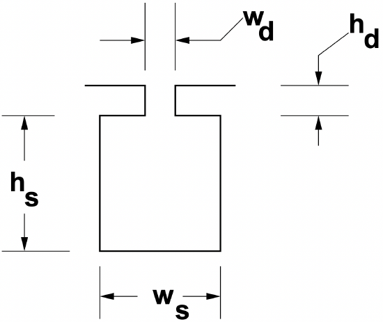Figure 5: Single Slot

Deep Slots

Now, suppose the slot is not small enough that diffusion effects can be ignored. The slot becomes “deep” to the extent that its depth is less than (or even comparable to) the skin depth for conduction at slip frequency. Conduction in this case may be represented by using the Diffusion Equation:

\(\ \nabla^{2} \bar{H}=\mu_{0} \sigma \frac{\partial \bar{H}}{\partial t}\)

In the steady state, and assuming that only cross-slot flux (in the y direction) is important, and the only variation that is important is in the radial (x) direction:

\(\ \frac{\partial^{2} H_{y}}{\partial x^{2}}=j \omega_{s} \mu_{0} \sigma H_{y}\)

This is solved by solutions of the form:

\(\ H_{y}=H_{\pm} e^{\pm(1+j) \frac{x}{\delta}}\)

where the skin depth is

\(\ \delta=\sqrt{\frac{2}{\omega_{s} \mu_{0} \sigma}}\)

Since \(\ H_{y}\) must vanish at the bottom of the slot, it must take the form:

\(\ H_{y}=H_{\operatorname{top}} \frac{\sinh (1+j) \frac{x}{\delta}}{\sinh (1+j) \frac{h_{s}}{\delta}}\)

Since current is the curl of magnetic field,

\(\ J_{z}=\sigma E_{z}=\frac{\partial H_{y}}{\partial x}=H_{\mathrm{top}} \frac{1+j}{\delta} \frac{\cosh (1+j) \frac{h_{s}}{\delta}}{\sinh (1+j) \frac{h_{s}}{\delta}}\)

Then slot impedance, per unit length, is:

\(\ Z_{\text {slot }}=\frac{1}{w_{s}} \frac{1+j}{\sigma \delta} \operatorname{coth}(1+j) \frac{h_{s}}{\delta}\)

Of course the impedance (purely reactive) due to the slot depression must be added to this. It is possible to extract the real and imaginary parts of this impedance (the process is algebraically a bit messy) to yield:

\(\ \begin{aligned}
R_{\text {slot }} &=\frac{1}{w_{s} \sigma \delta} \frac{\sinh 2 \frac{h_{s}}{\delta}+\sin 2 \frac{h_{s}}{\delta}}{\cosh 2 \frac{h_{s}}{\delta}-\cos 2 \frac{h_{s}}{\delta}} \\
L_{\text {slot }} &=\mu_{0} \frac{h_{d}}{w_{d}}+\frac{1}{\omega_{s}} \frac{1}{w_{s} \sigma \delta} \frac{\sinh 2 \frac{h_{s}}{\delta}-\sin 2 \frac{h_{s}}{\delta}}{\cosh 2 \frac{h_{s}}{\delta}-\cos 2 \frac{h_{s}}{\delta}}
\end{aligned}\)

Multiple Cages

The purpose of a “deep” slot is to improve starting performance of a motor. When the rotor is stationary, the frequency seen by rotor conductors is relatively high, and current crowding due to the skin effect makes rotor resistance appear to be high. As the rotor accelerates the frequency seen from the rotor drops, lessening the skin effect and making more use of the rotor conductor. This, then, gives the machine higher starting torque (requiring high resistance) without compromising running efficiency.

This effect can be carried even further by making use of multiple cages, such as is shown in Figure 6. Here there are two conductors in a fairly complex slot. Estimating the impedance of this slot is done in stages to build up an equivalent circuit.

Assume for the purposes of this derivation that each section of the multiple cage is small enough that currents can be considered to be uniform in each conductor. Then the bottom section may be represented as a resistance in series with an inductance:

\(\ R_{a}=\frac{1}{\sigma w_{1} h_{1}}\)

\(\ L_{a}=\frac{\mu_{0}}{3} \frac{h_{1}}{w_{1}}\)

The narrow slot section with no conductor between the top and bottom conductors will contribute an inductive impedance:

\(\ L_{s}=\mu_{0} \frac{h_{s}}{w_{s}}\)

The top conductor will have a resistance:

\(\ R_{b}=\frac{1}{\sigma w_{2} h_{2}}\)

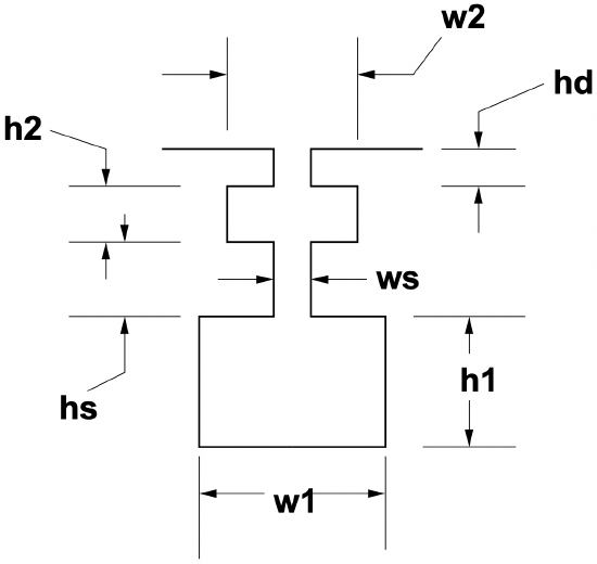Figure 6: Double Slot

Now, in the equivalent circuit, current flowing in the lower conductor will produce a magnetic field across this section, yielding a series inductance of

\(\ L_{b}=\mu_{0} \frac{h_{2}}{w_{2}}\)

By analogy with the bottom conductor, current in the top conductor flows through only one third of the inductance of the top section, leading to the equivalent circuit of Figure 7, once the inductance of the slot depression is added on:

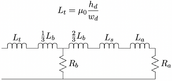Figure 7: Equivalent Circuit: Double Bar

Now, this rotor bar circuit fits right into the framework of the induction motor equivalent circuit, shown for the double cage case in Figure 8, with

\(\ \begin{aligned}
R_{2 a} &=\frac{12 l N_{S}^{2} k_{S}^{2}}{N_{R}} R_{a} \\
R_{2 b} &=\frac{12 l N_{S}^{2} k_{S}^{2}}{N_{R}} R_{b}
\end{aligned}\)

\(\ \begin{aligned}
X_{2 a} &=\omega \frac{12 l N_{S}^{2} k_{S}^{2}}{N_{R}}\left(\frac{2}{3} L_{b}+L_{s}+L_{a}\right) \\
X_{2 a} &=\omega \frac{12 l N_{S}^{2} k_{S}^{2}}{N_{R}}\left(L_{t}+\frac{1}{3} L_{b}\right)
\end{aligned}\)

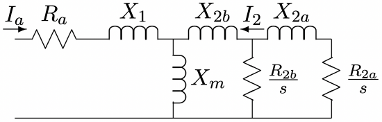Figure 8: Equivalent Circuit: Double Cage Rotor

Rotor End Ring Effects

It is necessary to correct for “end ring” resistance in the rotor. To do this, we note that the magnitude of surface current density in the rotor is related to the magnitude of individual bar current by:

\(\ I_{z}=K_{z} \frac{2 \pi R}{N_{R}}\label{115}\)

Current in the end ring is:

\(\ I_{R}=K_{z} \frac{R}{p}\label{116}\)

Then it is straightforward to calculate the ratio between power dissipated in the end rings to power dissipated in the conductor bars themselves, considering the ratio of current densities and volumes. Assuming that the bars and end rings have the same radial extent, the ratio of current densities is:

\(\ \frac{J_{R}}{J_{z}}=\frac{N_{R}}{2 \pi p} \frac{w_{r}}{l_{r}}\label{117}\)

where \(\ w_{r}\) is the average width of a conductor bar and \(\ l_{r}\) is the axial end ring length.

Now, the ratio of losses (and hence the ratio of resistances) is found by multiplying the square of current density ratio by the ratio of volumes. This is approximately:

\[\ \frac{R_{\text {end }}}{R_{\text {slot }}}=\left(\frac{N_{R}}{2 \pi p} \frac{w_{r}}{l_{r}}\right)^{2} 2 \frac{2 \pi R}{N_{R} l} \frac{l_{r}}{w_{r}}=\frac{N_{R} R w_{r}}{\pi l l_{r} p^{2}}\label{118} \]

Windage

Bearing friction, windage loss and fan input power are often regarded as elements of a “black art”. We approach them with some level of trepidation, for motor manufacturers seem to take a highly empirical view of these elements. What follows is an attempt to build reasonable but simple models for two effects: loss in the air gap due to windage and input power to the fan for cooling. Some caution is required here, for these elements of calculation have not been properly tested, although they seem to give reasonable numbers

The first element is gap windage loss. This is produced by shearing of the air in the relative rotation gap. It is likely to be a signifigant element only in machines with very narrow air gaps or very high surface speeds. But these include, of course, the high performance machines with which we are most interested. We approach this with a simple “couette flow” model. Air-gap shear loss is approximately:

\[\ P_{w}=2 \pi R^{4} \Omega^{3} l \rho_{a} f\label{119} \]

where \(\ \rho_{a}\) is the density of the air-gap medium (possibly air) and \(\ f\) is the friction factor, estimated by:

\[\ f=\frac{.0076}{R_{n}^{\frac{1}{4}}}\label{120} \]

and the Reynold’s Number \(\ R_{n}\) is

\[\ R_{n}=\frac{\Omega R g}{\nu_{\text {air }}}\label{121} \]

and \(\ \nu_{\text {air }}\) is the kinematic viscosity of the air-gap medium.

The second element is fan input power. We base an estimate of this on two hypotheses. The first of these is that the mass flow of air circulated by the fan can be calculated by the loss in the motor and an average temperature rise in the cooling air. The second hypothesis is the the pressure rise of the fan is established by the centrifugal pressure rise associated with the surface speed at the outside of the rotor. Taking these one at a time: If there is to be a temperature rise \(\ \Delta T\) in the cooling air, then the mass flow volume is:

\(\ \dot{m}=\frac{P_{d}}{C_{p} \Delta T}\)

and then volume flow is just

\(\ \dot{v}=\frac{\dot{m}}{\rho_{\text {air }}}\)

Pressure rise is estimated by centrifugal force:

\(\ \Delta P=\rho_{\text {air }}\left(\frac{\omega}{p} r_{\mathrm{fan}}\right)^{2}\)

then power is given by:

\(\ P_{\text {fan }}=\Delta P \dot{v}\)

For reference, the properties of air are:

Density	\(\ \rho_{\text {air }}\)	1.18	\(\ \mathrm{kg} / \mathrm{m}^{2}\)
Kinematic Viscosity	\\nu_{\text {air }}	\(\ 1.56 \times 10^{-5}\)	\(\ m^{2} / s e c\)
Heat Capacity	\(\ C_{p}\)	1005.7	\(\ \mathrm{J} / \mathrm{kg}\)

Magnetic Circuit Loss and Excitation

There will be some loss in the stator magnetic circuit due to eddy current and hysteresis effects in the core iron. In addition, particularly if the rotor and stator teeth are saturated there will be MMF expended to push flux through those regions. These effects are very difficult to estimate from first principles, so we resort to a simple model.

Assume that the loss in saturated steel follows a law such as:

\[\ P_{d}=P_{B}\left(\frac{\omega_{e}}{\omega_{B}}\right)^{\epsilon_{f}}\left(\frac{B}{B_{B}}\right)^{\epsilon_{b}}\label{122} \]

This is not too bad an estimate for the behavior of core iron. Typically, \(\ \epsilon_{f}\) is a bit less than two (between about 1.3 and 1.6) and \(\ \epsilon_{b}\) is a bit more than two (between about 2.1 and 2.4). Of course this model is good only for a fairly restricted range of flux density. Base dissipation is usually expressed in “watts per kilogram”, so we first compute flux density and then mass of the two principal components of the stator iron, the teeth and the back iron.

In a similar way we can model the exciting volt-amperes consumed by core iron by something like:

\[\ Q_{c}=\left(V a_{1}\left(\frac{B}{B_{B}}\right)^{\epsilon_{v 1}}+V a_{2}\left(\frac{B}{B_{B}}\right)^{\epsilon_{v 2}}\right) \frac{\omega}{\omega_{B}}\label{123} \]

This, too, is a form that appears to be valid for some steels. Quite obviously it may be necessary to develop different forms of curve ’fits’ for different materials.

Flux density (RMS) in the air-gap is:

\[\ B\_{r}=\frac{p V_{a}}{2 R l N_{a} k_{1} \omega_{s}}\label{124} \]

Then flux density in the stator teeth is:

\[\ B_{t}=B_{r} \frac{w_{t}+w_{1}}{w_{t}}\label{125} \]

where \(\ w_{t}\) is tooth width and \(\ w_{1}\) is slot top width. Flux in the back-iron of the core is

\[\ B_{c}=B_{r} \frac{R}{p d_{c}}\label{126} \]

where \(\ d_{c}\) is the radial depth of the core.

One way of handling this loss is to assume that the core handles flux corresponding to terminal voltage, add up the losses and then compute an equivalent resistance and reactance:

\(\ \begin{array}{l}
r_{c}=\frac{3\left|V_{a}\right|^{2}}{P_{\text {core }}} \\
x_{c}=\frac{3\left|V_{a}\right|^{2}}{Q_{\text {core }}}
\end{array}\)

then put this equivalent resistance in parallel with the air-gap reactance element in the equivalent circuit.