10.5: Induction Motor Speed Control

Introduction

The inherent attributes of induction machines make them very attractive for drive applications. They are rugged, economical to build and have no sliding contacts to wear. The difficulty with using induction machines in servomechanisms and variable speed drives is that they are “hard to control”, since their torque-speed relationship is complex and nonlinear. With, however, modern power electronics to serve as frequency changers and digital electronics to do the required arithmetic, induction machines are seeing increasing use in drive applications.

In this chapter we develop models for control of induction motors. The derivation is quite brief for it relies on what we have already done for synchronous machines. In this chapter, however, we will stay in “ordinary” variables, skipping the per-unit normalization.

Volts/Hz Control

Remembering that induction machines generally tend to operate at relatively low per unit slip, we might conclude that one way of building an adjustable speed drive would be to supply an induction motor with adjustable stator frequency. And this is, indeed, possible. One thing to remember is that flux is inversely proportional to frequency, so that to maintain constant flux one must make stator voltage proportional to frequency (hence the name “constant volts/Hz”). However, voltage supplies are always limited, so that at some frequency it is necessary to switch to constant voltage control. The analogy to DC machines is fairly direct here: below some “base” speed, the machine is controlled in constant flux (“volts/Hz”) mode, while above the base speed, flux is inversely proportional to speed. It is easy to see that the maximum torque is then inversely to the square of flux, or therefore to the square of frequency.

To get a first-order picture of how an induction machine works at adjustable speed, start with the simplified equivalent network that describes the machine, as shown in Figure 9

Earlier in this chapter, it was shown that torque can be calculated by finding the power dissipated in the virtual resistance \(\ R_{2} / s\) and dividing by electrical speed. For a three phase machine, and assuming we are dealing with RMS magnitudes:

\(\ T_{e}=3 \frac{p}{\omega}\left|I_{2}\right|^{2} \frac{R_{2}}{s}\)

where \(\ \omega\) is the electrical frequency and \(\ p\) is the number of pole pairs. It is straightforward to find \(\ I_{2}\) using network techniques. As an example, Figure 10 shows a series of torque/speed curves for

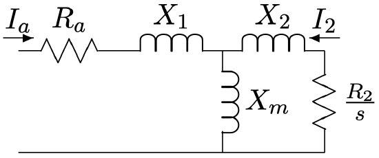Figure 9: Equivalent Circuit

an induction machine operated with a wide range of input frequencies, both below and above its “base” frequency. The parameters of this machine are:

Number of Phases	3
Number of Pole Pairs	3
RMS Terminal Voltage (line-line)	230
Frequency (Hz)	60
Stator Resistance \(\ R_{1}\)	.06 Ω
Rotor Resistance \(\ R_{2}\)	.055 Ω
Stator Leakage \(\ X_{1}\)	.34 Ω
Rotor Leakage \(\ X_{2}\)	.33 Ω
Magnetizing Reactance \(\ X_{m}\)	10.6 Ω

Strategy for operating the machine is to make terminal voltage magnitude proportional to frequency for input frequencies less than the “Base Frequency”, in this case 60 Hz, and to hold voltage constant for frequencies above the “Base Frequency”.

For high frequencies the torque production falls fairly rapidly with frequency (as it turns out, it is roughly proportional to the inverse of the square of frequency). It also falls with very low frequency because of the effects of terminal resistance. We will look at this next.

Idealized Model: No Stator Resistance

Ignore, for the moment, \(\ R_{1}\). An equivalent circuit is shown in Figure 11. It is fairly easy to show that, from the rotor, the combination of source, armature leakage and magnetizing branch can be replaced by its equivalent circuit, as shown in in Figure 12.

In the circuit of Figure 12, the parameters are:

\(\ \begin{aligned}
V^{\prime} &=V \frac{X_{m}}{X_{m}+X_{1}} \\
X^{\prime} &=X_{m} \| X_{1}
\end{aligned}\)

If the machine is operated at variable frequency \(\ \omega\), but the reactance is established at frequency \(\ \omega_{B}\), current is:

\(\ \underline{I}=\frac{V^{\prime}}{j\left(X_{1}^{\prime}+X_{2}\right) \frac{\omega}{\omega_{B}}+\frac{R_{2}}{s}}\)

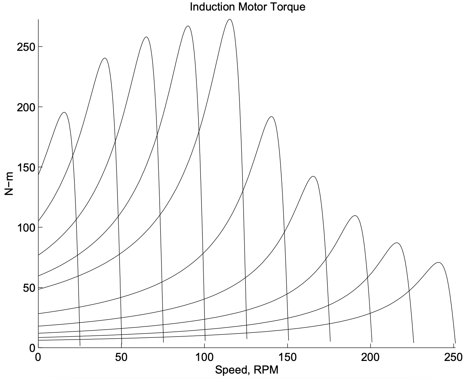Figure 10: Induction Machine Torque-Speed Curves

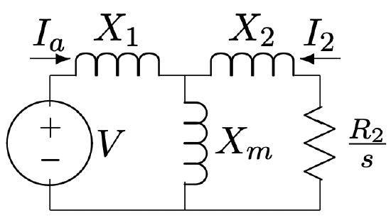Figure 11: Idealized Circuit: Ignore Armature Resistance

and then torque is

\(\ T_{e}=3\left|I_{2}\right|^{2} \frac{R_{2}}{s}=\frac{3 p}{\omega} \frac{\left|V^{\prime}\right|^{2} \frac{R_{2}}{s}}{\left(X_{1}^{\prime}+X_{2}\right)^{2}+\left(\frac{R_{2}}{s}\right)^{2}}\)

Now, if we note that what counts is the absolute slip of the rotor, we might define a slip with respect to base frequency:

\(\ s=\frac{\omega_{r}}{\omega}=\frac{\omega_{r}}{\omega_{B}} \frac{\omega_{B}}{\omega}=s_{B} \frac{\omega_{B}}{\omega}\)

Then, if we assume that voltage is applied proportional to frequency:

\(\ V^{\prime}=V_{0}^{\prime} \frac{\omega}{\omega_{B}}\)

and with a little manipulation, we get:

\(\ T_{e}=\frac{3 p}{\omega_{B}} \frac{\left|V_{0}^{\prime}\right|^{2} \frac{R_{2}}{s_{B}}}{\left(X_{1}^{\prime}+X_{2}\right)^{2}+\left(\frac{R_{2}}{s_{B}}\right)^{2}}\)

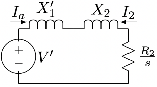Figure 12: Idealized Equivalent

This would imply that torque is, if voltage is proportional to frequency, meaning constant applied flux, dependent only on absolute slip. The torque-speed curve is a constant, dependent only on the difference between synchronous and actual rotor speed.

This is fine, but eventually, the notion of “volts per Hz” runs out because at some number of Hz, there are no more volts to be had. This is generally taken to be the “base” speed for the drive. Above that speed, voltage is held constant, and torque is given by:

\(\ T_{e}=\frac{3 p}{\omega_{B}} \frac{\left|V^{\prime}\right|^{2} \frac{R_{2}}{s_{B}}}{\left(X_{1}^{\prime}+X_{2}\right)^{2}+\left(\frac{R_{2}}{s_{B}}\right)^{2}}\)

The peak of this torque has a square-inverse dependence on frequency, as can be seen from Figure 13.

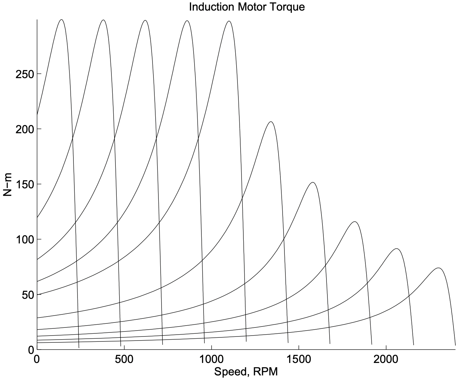Figure 13: Idealized Torque-Speed Curves: Zero Stator Resistance

Peak Torque Capability

Assuming we have a smart controller, we are interested in the actual capability of the machine. At some voltage and frequency, torque is given by:

\(\ T_{e}=3\left|I_{2}\right|^{2} \frac{R_{2}}{s}=\frac{3 \frac{p}{\omega}\left|V^{\prime}\right|^{2} \frac{R_{2}}{s}}{\left(\left(X_{1}^{\prime}+X_{2}\right)\left(\frac{\omega}{\omega_{B}}\right)\right)^{2}+\left(R_{1}^{\prime}+\frac{R_{2}}{s}\right)^{2}}\)

Now, we are interested in finding the peak value of that, which is given by the value of \(\ R_{2} s\) which maximizes power transfer to the virtual resistance. This is given by the matching condition:

\(\ \frac{R_{2}}{s}=\sqrt{R_{1}^{\prime 2}+\left(\left(X_{1}^{\prime}+X_{2}\right)\left(\frac{\omega}{\omega_{B}}\right)\right)^{2}}\)

Then maximum (breakdown) torque is given by:

\(\ T_{\max }=\frac{\frac{3 p}{\omega}\left|V^{\prime}\right|^{2} \sqrt{R_{1}^{\prime 2}+\left(\left(X_{1}^{\prime}+X_{2}\right)\left(\frac{\omega}{\omega_{B}}\right)\right)^{2}}}{\left(\left(X_{1}^{\prime}+X_{2}\right)\left(\frac{\omega}{\omega_{B}}\right)\right)^{2}+\left(R_{1}^{\prime}+\sqrt{R_{1}^{\prime 2}+\left(\left(X_{1}^{\prime}+X_{2}\right)\left(\frac{\omega}{\omega_{B}}\right)\right)^{2}}\right)^{2}}\)

This is plotted in Figure 14. Just as a check, this was calculated assuming \(\ R_{1}=0\), and the results are plotted in figure 15. This plot shows, as one would expect, a constant torque limit region to zero speed.

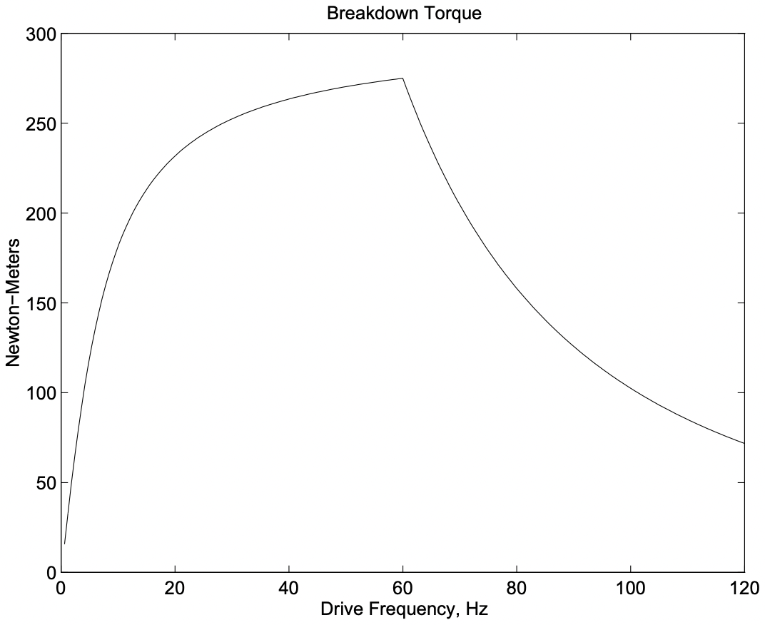Figure 14: Torque-Capability Curve For An Induction Motor

Field Oriented Control

One of the more useful impacts of modern power electronics and control technology has enabled us to turn induction machines into high performance servomotors. In this note we will develop a

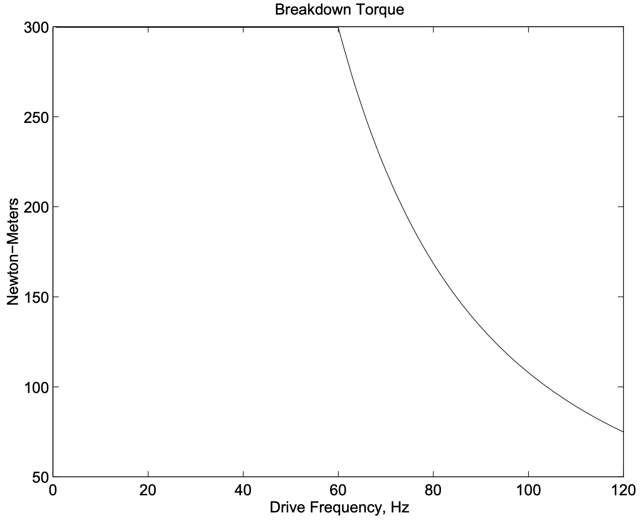Figure 15: Idealized Torque Capability Curve: Zero Stator Resistance

picture of how this is done. Quite obviously there are many details which we will not touch here. The objective is to emulate the performance of a DC machine, in which (as you will recall), torque is a simple function of applied current. For a machine with one field winding, this is simply:

\(\ T=G I_{f} I_{a}\)

This makes control of such a machine quite easy, for once the desired torque is known it is easy to translate that torque command into a current and the motor does the rest.

Of course DC (commutator) machines are, at least in large sizes, expensive, not particularly efficient, have relatively high maintenance requirements because of the sliding brush/commutator interface, provide environmental problems because of sparking and carbon dust and are environmentally sensitive. The induction motor is simpler and more rugged. Until fairly recently the induction motor has not been widely used in servo applications because it was thought to be ”hard to control”. As we will show, it does take a little effort and even some computation to do the controls right, but this is becoming increasingly affordable.

Elementary Model

We return to the elementary model of the induction motor. In ordinary variables, referred to the stator, the machine is described by flux-current relationships (in the d-q reference frame):

\(\ \begin{aligned}
\left[\begin{array}{c}
\lambda_{d S} \\
\lambda_{d R}
\end{array}\right] &=\left[\begin{array}{ll}
L_{S} & M \\
M & L_{R}
\end{array}\right]\left[\begin{array}{c}
i_{d S} \\
i_{d R}
\end{array}\right] \\
\left[\begin{array}{c}
\lambda_{q S} \\
\lambda_{q R}
\end{array}\right] &=\left[\begin{array}{ll}
L_{S} & M \\
M & L_{R}
\end{array}\right]\left[\begin{array}{c}
i_{q S} \\
i_{q R}
\end{array}\right]
\end{aligned}\)

Note the machine is symmetric (there is no saliency), and since we are referred to the stator, the stator and rotor self-inductances include leakage terms:

\(\ \begin{array}{l}
L_{S}=M+L_{S \ell} \\
L_{R}=M+L_{R \ell}
\end{array}\)

The voltage equations are:

\(\ \begin{aligned}
v_{d S} &=\frac{d \lambda_{d S}}{d t}-\omega \lambda_{q S}+r_{S} i_{d S} \\
v_{q S} &=\frac{d \lambda_{q S}}{d t}+\omega \lambda_{d S}+r_{S} i_{q S} \\
0 &=\frac{d \lambda_{d R}}{d t}-\omega_{s} \lambda_{q R}+r_{R} i_{d R} \\
0 &=\frac{d \lambda_{q R}}{d t}+\omega_{s} \lambda_{d R}+r_{R} i_{q R}
\end{aligned}\)

Note that both rotor and stator have “speed” voltage terms since they are both rotating with respect to the rotating coordinate system. The speed of the rotating coordinate system is w with respect to the stator. With respect to the rotor that speed is , where wm is the rotor mechanical speed. Note that this analysis does not require that the reference frame coordinate system speed w be constant.

Torque is given by:

\(\ T^{e}=\frac{3}{2} p\left(\lambda_{d S} i_{q S}-\lambda_{q S} i_{d S}\right)\)

Simulation Model

As a first step in developing a simulation model, see that the inversion of the flux-current relationship is (we use the d- axis since the q- axis is identical):

\(\ \begin{aligned}
i_{d S} &=\frac{L_{R}}{L_{S} L_{R}-M^{2}} \lambda_{d S}-\frac{M}{L_{S} L_{R}-M^{2}} \lambda_{d R} \\
i_{d R} &=\frac{M}{L_{S} L_{R}-M^{2}} \lambda_{d S}-\frac{L_{S}}{L_{S} L_{R}-M^{2}} \lambda_{d R}
\end{aligned}\)

Now, if we make the following definitions (the motivation for this should by now be obvious):

\(\ \begin{aligned}
X_{d} &=\omega_{0} L_{S} \\
X_{k d} &=\omega_{0} L_{R} \\
X_{a d} &=\omega_{0} M \\
X_{d}^{\prime} &=\omega_{0}\left(L_{S}-\frac{M^{2}}{L_{R}}\right)
\end{aligned}\)

the currents become:

\(\ \begin{aligned}
i_{d S} &=\frac{\omega_{0}}{X_{d}^{\prime}} \lambda_{d S}-\frac{X_{a d}}{X_{k d}} \frac{\omega_{0}}{X_{d}^{\prime}} \lambda_{d R} \\
i_{d R} &=\frac{X_{a d}}{X_{k d}} \frac{\omega_{0}}{X_{d}^{\prime}} \lambda_{d S}-\frac{X_{d}}{X_{d}^{\prime}} \frac{\omega_{0}}{X_{k d}} \lambda_{d R}
\end{aligned}\)

The q- axis is the same.

Torque may be, with these calculations for current, written as:

\(\ T_{e}=\frac{3}{2} p\left(\lambda_{d S} i_{q S}-\lambda_{q S} i_{d S}\right)=-\frac{3}{2} p \frac{\omega_{0} X_{a d}}{X_{k d} X_{d}^{\prime}}\left(\lambda_{d S} \lambda_{q R}-\lambda_{q S} \lambda_{d R}\right)\)

Note that the usual problems with ordinary variables hold here: the foregoing expression was written assuming the variables are expressed as peak quantities. If

RMS is used we must replace 3/2 by 3!

With these, the simulation model is quite straightforward. The state equations are:

\(\ \begin{array}{l}
\frac{d \lambda_{d S}}{d t}=V_{d S}+\omega \lambda_{q S}-R_{S} i_{d S} \\
\frac{d \lambda_{q S}}{d t}=V_{q S}-\omega \lambda_{d S}-R_{S} i_{q S} \\
\frac{d \lambda_{d R}}{d t}=\omega_{s} \lambda_{q R}-R_{R} i_{d R} \\
\frac{d \lambda_{q R}}{d t}=-\omega_{s} \lambda_{d R}-R_{S} i_{q R} \\
\frac{d \Omega_{m}}{d t}=\frac{1}{J}\left(T_{e}+T_{m}\right)
\end{array}\)

where the rotor frequency (slip frequency) is:

\(\ \omega_{s}=\omega-p \Omega_{m}\)

For simple simulations and constant excitaion frequency, the choice of coordinate systems is arbitrary, so we can choose something convenient. For example, we might choose to fix the coordinate system to a synchronously rotating frame, so that stator frequency \(\ \omega=\omega_{0}\). In this case, we could pick the stator voltage to lie on one axis or another. A common choice is \(\ V_{d}=0\) and \(\ V_{q}=V\).

Control Model

If we are going to turn the machine into a servomotor, we will want to be a bit more sophisticated about our coordinate system. In general, the principle of field-oriented control is much like emulating the function of a DC (commutator) machine. We figure out where the flux is, then inject current to interact most directly with the flux.

As a first step, note that because the two stator flux linkages are the sum of air-gap and leakage flux,

\(\ \begin{aligned}
\lambda_{d S} &=\lambda_{a g d}+L_{S \ell} i_{d S} \\
\lambda_{q S} &=\lambda_{a g q}+L_{S \ell} i_{q S}
\end{aligned}\)

This means that we can re-write torque as:

\(\ T^{e}=\frac{3}{2} p\left(\lambda_{a g d} i_{q S}-\lambda_{a g q} i_{d S}\right)\)

Next, note that the rotor flux is, similarly, related to air-gap flux:

\(\ \begin{aligned}
\lambda_{a g d} &=\lambda_{d R}-L_{R \ell} i_{d R} \\
\lambda_{a g q} &=\lambda_{q R}-L_{R \ell} i_{q R}
\end{aligned}\)

Torque now becomes:

\(\ T^{e}=\frac{3}{2} p\left(\lambda_{d R} i_{q S}-\lambda_{q R} i_{d S}\right)-\frac{3}{2} p L_{R \ell}\left(i_{d R} i_{q S}-i_{q R} i_{d S}\right)\)

Now, since the rotor currents could be written as:

\(\ \begin{array}{l}
i_{d R}=\frac{\lambda_{d R}}{L_{R}}-\frac{M}{L_{R}} i_{d S} \\
i_{q R}=\frac{\lambda_{q R}}{L_{R}}-\frac{M}{L_{R}} i_{q S}
\end{array}\)

That second term can be written as:

\(\ i_{d R} i_{q S}-i_{q R} i_{d S}=\frac{1}{L_{R}}\left(\lambda_{d R} i_{q S}-\lambda_{q R} i_{d S}\right)\)

So that torque is now:

\(\ T^{e}=\frac{3}{2} p\left(1-\frac{L_{R \ell}}{L_{R}}\right)\left(\lambda_{d R} i_{q S}-\lambda_{q R} i_{d S}\right)=\frac{3}{2} p \frac{M}{L_{R}}\left(\lambda_{d R} i_{q S}-\lambda_{q R} i_{d S}\right)\)

Field-Oriented Strategy

What is done in field-oriented control is to establish a rotor flux in a known position (usually this position is the d- axis of the transformation) and then put a current on the orthogonal axis (where it will be most effective in producing torque). That is, we will attempt to set

\(\ \begin{array}{l}
\lambda_{d R}=\Lambda_{0} \\
\lambda_{q R}=0
\end{array}\)

Then torque is produced by applying quadrature-axis current:

\(\ T^{e}=\frac{3}{2} p \frac{M}{L_{R}} \Lambda_{0} i_{q S}\)

The process is almost that simple. There are a few details involved in figuring out where the quadrature axis is and how hard to drive the direct axis (magnetizing) current.

Now, suppose we can succeed in putting flux on the right axis, so that \(\ \lambda_{q R}=0\), then the two rotor voltage equations are:

\(\ \begin{aligned}
0 &=\frac{d \lambda_{d R}}{d t}-\omega_{s} \lambda_{q R}+r_{R} I_{d R} \\
0 &=\frac{d \lambda_{q R}}{d t}+\omega_{s} \lambda_{d R}+r_{R} I_{q R}
\end{aligned}\)

Now, since the rotor currents are:

\(\ \begin{aligned}
i_{d R} &=\frac{\lambda_{d R}}{L_{R}}-\frac{M}{L_{R}} i_{d S} \\
i_{q R} &=\frac{\lambda_{q R}}{L_{R}}-\frac{M}{L_{R}} i_{q S}
\end{aligned}\)

The voltage expressions become, accounting for the fact that there is no rotor quadrature axis flux:

\(\ \begin{aligned}
0 &=\frac{d \lambda_{d R}}{d t}+r_{R}\left(\frac{\lambda_{d R}}{L_{R}}-\frac{M}{L_{R}} i_{d S}\right) \\
0 &=\omega_{s} \lambda_{d R}-r_{R} \frac{M}{L_{R}} i_{q S}
\end{aligned}\)

Noting that the rotor time constant is

\(\ T_{R}=\frac{L_{R}}{r_{R}}\)

we find:

\(\ \begin{aligned}
T_{R} \frac{d \lambda_{d R}}{d t}+\lambda_{d R} &=M i_{d S} \\
\omega_{s} &=\frac{M}{T_{R}} \frac{i_{q S}}{\lambda_{d R}}
\end{aligned}\)

The first of these two expressions describes the behavior of the direct-axis flux: as one would think, it has a simple first-order relationship with direct-axis stator current. The second expression, which describes slip as a function of quadrature axis current and direct axis flux, actually describes how fast to turn the rotating coordinate system to hold flux on the direct axis.

Now, a real machine application involves phase currents \(\ i_{a}\), \(\ i_{b}\) and \(\ i_{c}\), and these must be derived from the model currents \(\ i_{d S}\) and \(\ i_{q s}\). This is done with, of course, a mathematical operation which uses a transformation angle \(\ \theta\). And that angle is derived from the rotor mechanical speed and computed slip:

\(\ \theta=\int\left(p \omega_{m}+\omega_{s}\right) d t\)

A generally good strategy to make this sort of system work is to measure the three phase currents and derive the direct- and quadrature-axis currents from them. A good estimate of direct-axis flux is made by running direct-axis flux through a first-order filter. The tricky operation involves dividing quadrature axis current by direct axis flux to get slip, but this is now easily done numerically (as are the trigonometric operations required for the rotating coordinate system transformation). An elmentary block diagram of a (possbly) plausible scheme for this is shown in Figure 16.

In this picture we start with commanded values of direct- and quadrature- axis currents, corresponding to flux and torque, respectively. These are translated by a rotating coordinate transformation into commanded phase currents. That transformation (simply the inverse Park’s transform) uses the angle q derived as part of the scheme. In some (cheap) implementations of this scheme the commanded currents are used rather than the measured currents to establish the flux and slip.

We have shown the commanded currents \(\ i_{a}^{*}\), etc. as inputs to an “Amplifier”. This might be implemented as a PWM current-source, for example, and a tight loop here results in a rather high performance servo system.

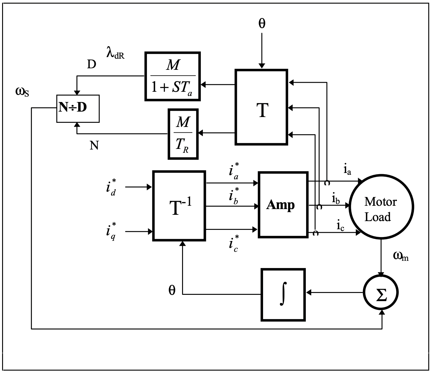Figure 16: Field Oriented Controller

References

Equation \ref{1} P.L. Alger, “Induction Machines”, Gordon and Breach, 1969

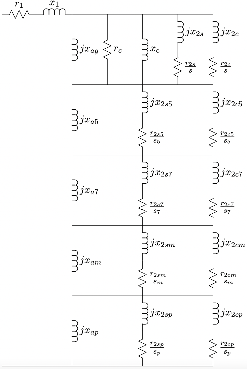Figure 17: Extended Equivalent Circuit