6.4: Dependent Sources
- Page ID
- 25275

\( \newcommand{\vecs}[1]{\overset { \scriptstyle \rightharpoonup} {\mathbf{#1}} } \)
\( \newcommand{\vecd}[1]{\overset{-\!-\!\rightharpoonup}{\vphantom{a}\smash {#1}}} \)
\( \newcommand{\dsum}{\displaystyle\sum\limits} \)
\( \newcommand{\dint}{\displaystyle\int\limits} \)
\( \newcommand{\dlim}{\displaystyle\lim\limits} \)
\( \newcommand{\id}{\mathrm{id}}\) \( \newcommand{\Span}{\mathrm{span}}\)
( \newcommand{\kernel}{\mathrm{null}\,}\) \( \newcommand{\range}{\mathrm{range}\,}\)
\( \newcommand{\RealPart}{\mathrm{Re}}\) \( \newcommand{\ImaginaryPart}{\mathrm{Im}}\)
\( \newcommand{\Argument}{\mathrm{Arg}}\) \( \newcommand{\norm}[1]{\| #1 \|}\)
\( \newcommand{\inner}[2]{\langle #1, #2 \rangle}\)
\( \newcommand{\Span}{\mathrm{span}}\)
\( \newcommand{\id}{\mathrm{id}}\)
\( \newcommand{\Span}{\mathrm{span}}\)
\( \newcommand{\kernel}{\mathrm{null}\,}\)
\( \newcommand{\range}{\mathrm{range}\,}\)
\( \newcommand{\RealPart}{\mathrm{Re}}\)
\( \newcommand{\ImaginaryPart}{\mathrm{Im}}\)
\( \newcommand{\Argument}{\mathrm{Arg}}\)
\( \newcommand{\norm}[1]{\| #1 \|}\)
\( \newcommand{\inner}[2]{\langle #1, #2 \rangle}\)
\( \newcommand{\Span}{\mathrm{span}}\) \( \newcommand{\AA}{\unicode[.8,0]{x212B}}\)
\( \newcommand{\vectorA}[1]{\vec{#1}} % arrow\)
\( \newcommand{\vectorAt}[1]{\vec{\text{#1}}} % arrow\)
\( \newcommand{\vectorB}[1]{\overset { \scriptstyle \rightharpoonup} {\mathbf{#1}} } \)
\( \newcommand{\vectorC}[1]{\textbf{#1}} \)
\( \newcommand{\vectorD}[1]{\overrightarrow{#1}} \)
\( \newcommand{\vectorDt}[1]{\overrightarrow{\text{#1}}} \)
\( \newcommand{\vectE}[1]{\overset{-\!-\!\rightharpoonup}{\vphantom{a}\smash{\mathbf {#1}}}} \)
\( \newcommand{\vecs}[1]{\overset { \scriptstyle \rightharpoonup} {\mathbf{#1}} } \)
\( \newcommand{\vecd}[1]{\overset{-\!-\!\rightharpoonup}{\vphantom{a}\smash {#1}}} \)
\(\newcommand{\avec}{\mathbf a}\) \(\newcommand{\bvec}{\mathbf b}\) \(\newcommand{\cvec}{\mathbf c}\) \(\newcommand{\dvec}{\mathbf d}\) \(\newcommand{\dtil}{\widetilde{\mathbf d}}\) \(\newcommand{\evec}{\mathbf e}\) \(\newcommand{\fvec}{\mathbf f}\) \(\newcommand{\nvec}{\mathbf n}\) \(\newcommand{\pvec}{\mathbf p}\) \(\newcommand{\qvec}{\mathbf q}\) \(\newcommand{\svec}{\mathbf s}\) \(\newcommand{\tvec}{\mathbf t}\) \(\newcommand{\uvec}{\mathbf u}\) \(\newcommand{\vvec}{\mathbf v}\) \(\newcommand{\wvec}{\mathbf w}\) \(\newcommand{\xvec}{\mathbf x}\) \(\newcommand{\yvec}{\mathbf y}\) \(\newcommand{\zvec}{\mathbf z}\) \(\newcommand{\rvec}{\mathbf r}\) \(\newcommand{\mvec}{\mathbf m}\) \(\newcommand{\zerovec}{\mathbf 0}\) \(\newcommand{\onevec}{\mathbf 1}\) \(\newcommand{\real}{\mathbb R}\) \(\newcommand{\twovec}[2]{\left[\begin{array}{r}#1 \\ #2 \end{array}\right]}\) \(\newcommand{\ctwovec}[2]{\left[\begin{array}{c}#1 \\ #2 \end{array}\right]}\) \(\newcommand{\threevec}[3]{\left[\begin{array}{r}#1 \\ #2 \\ #3 \end{array}\right]}\) \(\newcommand{\cthreevec}[3]{\left[\begin{array}{c}#1 \\ #2 \\ #3 \end{array}\right]}\) \(\newcommand{\fourvec}[4]{\left[\begin{array}{r}#1 \\ #2 \\ #3 \\ #4 \end{array}\right]}\) \(\newcommand{\cfourvec}[4]{\left[\begin{array}{c}#1 \\ #2 \\ #3 \\ #4 \end{array}\right]}\) \(\newcommand{\fivevec}[5]{\left[\begin{array}{r}#1 \\ #2 \\ #3 \\ #4 \\ #5 \\ \end{array}\right]}\) \(\newcommand{\cfivevec}[5]{\left[\begin{array}{c}#1 \\ #2 \\ #3 \\ #4 \\ #5 \\ \end{array}\right]}\) \(\newcommand{\mattwo}[4]{\left[\begin{array}{rr}#1 \amp #2 \\ #3 \amp #4 \\ \end{array}\right]}\) \(\newcommand{\laspan}[1]{\text{Span}\{#1\}}\) \(\newcommand{\bcal}{\cal B}\) \(\newcommand{\ccal}{\cal C}\) \(\newcommand{\scal}{\cal S}\) \(\newcommand{\wcal}{\cal W}\) \(\newcommand{\ecal}{\cal E}\) \(\newcommand{\coords}[2]{\left\{#1\right\}_{#2}}\) \(\newcommand{\gray}[1]{\color{gray}{#1}}\) \(\newcommand{\lgray}[1]{\color{lightgray}{#1}}\) \(\newcommand{\rank}{\operatorname{rank}}\) \(\newcommand{\row}{\text{Row}}\) \(\newcommand{\col}{\text{Col}}\) \(\renewcommand{\row}{\text{Row}}\) \(\newcommand{\nul}{\text{Nul}}\) \(\newcommand{\var}{\text{Var}}\) \(\newcommand{\corr}{\text{corr}}\) \(\newcommand{\len}[1]{\left|#1\right|}\) \(\newcommand{\bbar}{\overline{\bvec}}\) \(\newcommand{\bhat}{\widehat{\bvec}}\) \(\newcommand{\bperp}{\bvec^\perp}\) \(\newcommand{\xhat}{\widehat{\xvec}}\) \(\newcommand{\vhat}{\widehat{\vvec}}\) \(\newcommand{\uhat}{\widehat{\uvec}}\) \(\newcommand{\what}{\widehat{\wvec}}\) \(\newcommand{\Sighat}{\widehat{\Sigma}}\) \(\newcommand{\lt}{<}\) \(\newcommand{\gt}{>}\) \(\newcommand{\amp}{&}\) \(\definecolor{fillinmathshade}{gray}{0.9}\)A dependent source is a current or voltage source whose value is not fixed. Instead, the value depends on some other circuit current or voltage. The general form for the value of a dependent source is \(N = kM\) where \(M\) and \(N\) are currents and/or voltages and \(k\) is the proportionality constant. For example, the value of a dependent voltage source may be a function of a current, so instead of the source being equal to, say, 10 volts, it could be equal to twenty times the current passing through a particular resistor, or \(v = 20i\).
There are four possible dependent sources: They are the voltage-controlled voltage source (VCVS), the voltage-controlled current source (VCCS), the current-controlled voltage source (CCVS), and the current-controlled current source (CCCS). The source and control parameters are the same for both the VCVS and the CCCS so \(k\) has no units, although it may be given as volts/volt and amps/amp, respectively. For the VCCS and CCVS, \(k\) has units of amps/volt and volts/amp, respectively. These are referred to as the transresistance and transconductance of the sources with units of ohms and siemens.
The schematic symbols for dependent or controlled sources are usually drawn using a diamond instead of a circle. Also, for simulators, there will be a secondary connection for the controlling current or voltage. Examples of voltage-controlled and current-controlled sources are shown in Figure \(\PageIndex{1}\). On each of these symbols, the control element is shown to the left of the source.
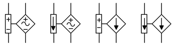
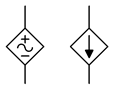
The control portion can be thought of as a connection for a voltmeter or ammeter which senses the control parameter. These sensing connections are not always drawn on a schematic. Instead, the source simply may be labeled as a function, as in \(v = 0.02 i_X\) where \(i_X\) is the controlling current. These simpler controlled sources are shown in Figure \(\PageIndex{2}\) and are typical in electronic schematics and texts. In some cases, these sources are drawn with a circle instead of a diamond. Also, the sine wave shape shown here is often omitted from the inside of symbol, however, current sources are always drawn with an arrow pointing in the reference direction and voltages sources always include the reference polarity.
Dependent sources are not “off-the-shelf” items in the same way that a battery or signal generator are. Rather, dependent sources are used to model the behavior of more complex devices. For example, a bipolar junction transistor commonly is modeled as a CCCS while a field effect transistor may be modeled as a VCCS. Similarly, many amplifier circuits are modeled as VCVS systems. Solutions for circuits using dependent sources follow along the lines of those established for independent sources (i.e., the application of Ohm's law, KVL, KCL, etc.), however, the sources are now dependent on the remainder of the circuit which tends to complicate the analysis. In general, there are two possible circuit configurations for dependent sources: isolated and coupled. An example of the isolated form is shown in Figure \(\PageIndex{3}\).
In this example, the dependent source (center, a CCVS) does not interact with the sub-circuit on the left driven by the independent source \(E\). Thus it can be analyzed as two separate circuits as shown in Figure \(\PageIndex{4}\).
Solutions for this form are relatively straightforward. The control value for the dependent source can be computed directly using standard techniques. Then this value is substituted into the dependent source and the analysis continues as normal. Sometimes it is convenient if the solution for a particular voltage or current is defined in terms of the control parameter rather than as a specific value (e.g., the current through a particular component might be 75 \(i_1\) instead of just 1 milliamp).
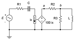
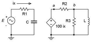
The second type of circuit (coupled) is somewhat more complex in that the dependent source can affect the parameter that controls the dependent source. An example is shown in Figure \(\PageIndex{5}\).
In this example it should be obvious that the voltage from the dependent source can affect the voltage at node \(a\), and it is this very voltage that defines \(i_x\), which in turn sets up the value of the dependent source. As far as analysis is concerned, either mesh or nodal can be used. The dependent source(s) will contribute terms that include the controlling parameter(s) so some additional effort will be required. To illustrate the technique, consider the circuit of Figure \(\PageIndex{6}\). We shall use the general method of nodal analysis.
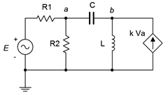
We begin by defining current directions. Assume that the currents through \(R_1\) and \(C\) are flowing into node \(a\), the current through \(R_2\) is flowing out of node \(a\), and the current through \(L\) is flowing out of node \(b\). We shall number the branch currents to reflect the associated components, from left to right. The resulting KCL equations are:
\[\sum i_{in} = \sum i_{out} \nonumber \]
\[\text{Node } a: i_1 +i_3 = i_2 \nonumber \]
\[\text{Node } b: k v_a = i_3 +i_4 \nonumber \]
The currents are then described by their Ohm's law equivalents:
\[\text{Node } a: \frac{E−v_a}{R_1} + \frac{v_b−v_a}{− jX_C} = \frac{v_a}{R_2} \nonumber \]
\[\text{Node } b: k v_a = \frac{v_b−v_a}{R_2} + \frac{v_b}{jX_L} \nonumber \]
Expanding terms yields:
\[\text{Node } a: \frac{E}{R_1} − \frac{v_a}{R_1} + \frac{v_b}{− jX_C} − \frac{v_a}{− jX_C} = \frac{v_a}{R_2} \nonumber \]
\[\text{Node } b: k v_a = \frac{v_b}{R_2} − \frac{v_a}{R_2} + \frac{v_b}{jX_L} \nonumber \]
Collecting terms and simplifying yields:
\[\text{Node } a : \frac{E}{R_1} = \left( \frac{1}{R_1} + \frac{1}{R_2} + \frac{1}{− jX_C} \right) v_a − \frac{1}{− jX_C} v_b \nonumber \]
\[\text{Node } b: 0 = − \left( k + \frac{1}{R_2} \right) v_a + \left( \frac{1}{R_2} + \frac{1}{jX_L} \right) v_b \nonumber \]
At this point, the component values and independent source value would be inserted into the equations and the system solved.
Finally, referring back to the prior chapter, it is possible to perform source conversions on dependent sources, within limits. The new source will remain a dependent source (e.g., VCVS to VCCS). This process is not applicable if the control parameter directly involves the internal impedance (i.e., is its voltage or current).
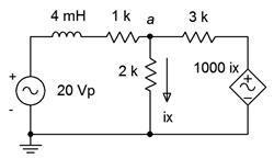
Example 6.11
For the circuit shown in Figure \(\PageIndex{7}\), determine \(v_c\) if the source is \(1\angle 0^{\circ}\) volt peak.

This is an example of the isolated or uncoupled dependent source. The value of the dependent current source is 30 times the value of the current labeled \(i_x\), which is the current flowing through the \(−j2 k\Omega\) capacitive reactance. We can find this current first and then determine the resulting value of the dependent source. The analysis will require nothing beyond basic series-parallel techniques. We will number the components from left to right.
The current \(i_x\) is found via Ohm's law:
\[i_x = \frac{E}{− jX_{C1}} \nonumber \]
\[i_x = \frac{1\angle 0^{\circ} V}{− j 2 k\Omega} \nonumber \]
\[i_x = 0.5E-3\angle 90 ^{\circ} A \nonumber \]
The dependent source is 30 times this value, or \(15E−3\angle 90^{\circ}\) amps. Given the reference direction of this source, the current is flowing upwards through the 65 k\(\Omega\) resistor and parallel \(−j50 k\Omega\) capacitor. This establishes \(v_c\) as negative. Multiplying \(i_x\) by the parallel impedance yields the desired voltage.
\[Z_{RC} = \frac{R_3 \times jX_{C2}}{R_3 − jX_{C2}} \nonumber \]
\[Z_{RC} = \frac{65k \Omega \times (− j50 k \Omega)}{65 k\Omega − j 50 k \Omega} \nonumber \]
\[Z_{RC} = 39.6E3\angle −52.4^{\circ} \Omega \nonumber \]
\[v_c = −i_x \times Z_{RC} \nonumber \]
\[v_c =−15E-3\angle 90^{\circ} \Omega \times 39.6E3\angle −52.4^{\circ} \Omega \nonumber \]
\[v_c = 594\angle −142.4 ^{\circ}V \nonumber \]
The next example features a coupled configuration solved using nodal analysis.
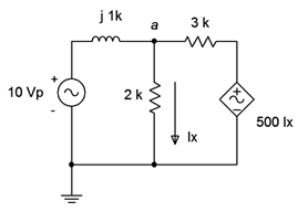
Example 6.12
In the circuit of Figure \(\PageIndex{8}\), determine \(v_a\). \(E =20\angle 0^{\circ}\) volts peak at 50 kHz.
In this circuit we have a current controlled voltage source, or CCVS. The proper unit for the constant of 1000 is ohms (volts over amps). First, we need to determine the reactance value for the inductor.
\[X_L = 2\pi f L \nonumber \]
\[X_L = 2\pi 50 kHz 4mH \nonumber \]
\[X_L = j 1257\Omega \nonumber \]
There is only one node of interest here (\(a\)) so we will only need one KCL equation. The sole unknown is \(v_a\). Let's assume that the reference directions of the currents flowing through the 1 k\(\Omega\) and 3 k\(\Omega\) resistors are entering node \(a\). We'll call these \(i_1\) and \(i_2\), respectively. The exiting current is \(i_x\).
The KCL summation is:
\[\sum i_{in} = \sum i_{out} \nonumber \]
\[i_1+i_2 = i_x \nonumber \]
This is expanded using Ohm's law (in several steps, for clarity).
\[i_x = i_1+i_2 \nonumber \]
\[\frac{v_a}{R_2} = \frac{E −v_a}{R_1+jX_L} + \frac{1000(\Omega)i_x−v_a}{R_3} \nonumber \]
\[\frac{v_a}{2 k\Omega} = \frac{20\angle 0^{\circ} V−v_a}{1k+j 1257\Omega} + \frac{1000 (\Omega)i_x−v_a}{3k \Omega} \nonumber \]
\[\frac{20\angle 0^{\circ} V}{1 k+j 1257\Omega} = \frac{v_a}{1k+j 1257\Omega} + \frac{v_a}{2k \Omega} + \frac{v_a}{3k \Omega} − \frac{1000(\Omega)i_x}{3k \Omega} \nonumber \]
\[12.45\angle −51.5^{\circ} A = \frac{v_a}{1k+j 1257\Omega} + \frac{v_a}{2 k\Omega} + \frac{v_a}{3k \Omega} − \frac{1000(\Omega) v_a}{2k \Omega \times 3k \Omega} \nonumber \]
\[12.45\angle −51.5^{\circ} A = \frac{v_a}{1k+j 1257\Omega} + \frac{v_a}{2k \Omega} + \frac{v_a}{3k\Omega} − \frac{v_a}{6k \Omega} \nonumber \]
\[12.45\angle −51.5^{\circ} A = \left( \frac{1}{1 k+j1257\Omega} + \frac{1}{2 k\Omega} + \frac{1}{3k \Omega} − \frac{1}{6 k\Omega} \right) v_a \nonumber \]
\[12.45\angle −51.5^{\circ} A = 1.161E-3\angle −24.8^{\circ} S v_a \nonumber \]
\[v_a = 10.7 \angle −26.7^{\circ} V \nonumber \]
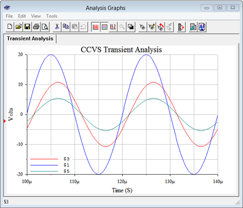
Computer Simulation
For verification, the dependent source circuit of Example \(\PageIndex{2}\) is entered into a simulator as shown in Figure \(\PageIndex{9}\). The results are shown in Figure \(\PageIndex{10}\).
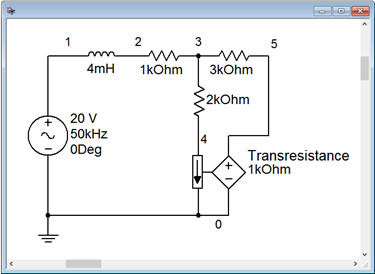
Note the connection to sense the current \(i_x\). It is inserted just like an ammeter. As mentioned previously, the constant for the dependent source is a transresistance and has units of ohms. A transient analysis is run the circuit, plotting the independent source, \(E\), as node 1 (blue), and \(v_a\) as node 3 (red). Both the amplitude and lagging phase shift line up nicely with the computed result. The voltage of the dependent source is also plotted as node 5 (green). Verifying this potential is left as an exercise.