
6.6: Exercises
- Page ID
- 25277

Analysis
(All source values are in amps or volts unless specified otherwise)
1. Given the circuit in Figure \(\PageIndex{1}\), use nodal analysis to determine \(v_c\). \(I_1 = 3\angle 0^{\circ}\), \(I_2 = 0.9\angle 0^{\circ}\).
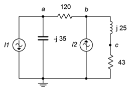
Figure \(\PageIndex{1}\)
2. Use nodal analysis to find the current through the 120 \(\Omega\) resistor in the circuit of Figure \(\PageIndex{2}\). \(I_1 = 0.5\angle 90^{\circ}\), \(I_2 = 1.6\angle 0^{\circ}\).
3. Use nodal analysis to find the current through the 43 \(\Omega\) resistor in the circuit of Figure \(\PageIndex{2}\). The sources are in phase.
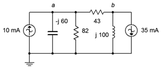
Figure \(\PageIndex{2}\)
4. Given the circuit in Figure \(\PageIndex{2}\), use nodal analysis to determine \(v_b\). The sources are in phase.
5. Given the circuit in Figure \(\PageIndex{3}\), determine \(v_c\). \(I_1 = 3\angle 0^{\circ}\), \(I_2 = 2\angle 0^{\circ}\).
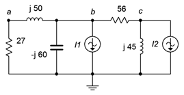
Figure \(\PageIndex{3}\)
6. Use nodal analysis to find the current through the \(j45 \Omega\) inductor in the circuit of Figure \(\PageIndex{3}\). \(I_1 = 2\angle 0^{\circ}\), \(I_2 = 1.5\angle 60^{\circ}\).
7. Use nodal analysis to find the current through the 4 \(\Omega\) resistor in the circuit of Figure \(\PageIndex{4}\). \(I_1 = 1\angle 45^{\circ}\), \(I_2 = 2\angle 45^{\circ}\).
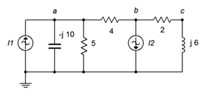
Figure \(\PageIndex{4}\)
8. Given the circuit in Figure \(\PageIndex{4}\), use nodal analysis to determine \(v_c\). \(I_1 = 6\angle 30^{\circ}\), \(I_2 = 4\angle 0^{\circ}\).
9. Given the circuit in Figure \(\PageIndex{5}\), use nodal analysis to determine \(v_{ac}\). \(I_1 = 10\angle 0^{\circ}\), \(I_2 = 6\angle 0^{\circ}\).
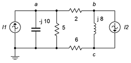
Figure \(\PageIndex{5}\)
10. Use nodal analysis to find the current through the \(j8 \Omega\) inductor in the circuit of Figure \(\PageIndex{5}\). \(I_1 = 3\angle 0^{\circ}\), \(I2 = 5\angle 30^{\circ}\).
11. Use nodal analysis to find the current through the 22 \(\Omega\) resistor in the circuit of Figure \(\PageIndex{6}\). \(I_1 = 800E−3\angle 0^{\circ}\), \(I_2 = 2.5\angle 0^{\circ}\), \(I_3 = 2\angle 20^{\circ}\).
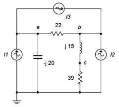
Figure \(\PageIndex{6}\)
12. Given the circuit in Figure \(\PageIndex{6}\), use nodal analysis to determine \(v_c\). \(I_1 = 4\angle 90^{\circ}\), \(I_2 = 10\angle 120^{\circ}\), \(I_3 = 5\angle 0^{\circ}\).
13. Given the circuit in Figure \(\PageIndex{7}\), use nodal analysis to determine \(v_c\). \(I_1 = 3E−3\angle 0^{\circ}\), \(I_2 = 10E−3\angle 0^{\circ}\), \(I_3 = 2E−3\angle 0^{\circ}\).
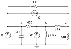
Figure \(\PageIndex{7}\)
14. Use nodal analysis to find the current through the \(−j2\) k\(\Omega\) capacitor in the circuit of Figure \(\PageIndex{7}\). \(I_1 = 1E−3\angle 0^{\circ}\), \(I_2 = 5E−3\angle 0^{\circ}\), \(I_3 = 6E−3\angle −90^{\circ}\).
15. Use nodal analysis to find the current through the 3.3 k\(\Omega\) resistor in the circuit of Figure \(\PageIndex{8}\). \(E = 36\angle 0^{\circ}\), \(I = 4E−3\angle −120^{\circ}\).
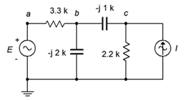
Figure \(\PageIndex{8}\)
16. Given the circuit in Figure \(\PageIndex{8}\), write the node equations and determine \(v_c\). \(E = 18\angle 0^{\circ}\), \(I = 7.5E−3\angle −30^{\circ}\).
17. Given the circuit in Figure \(\PageIndex{9}\), use nodal analysis to determine \(v_c\). \(E = 40\angle 180^{\circ}\), \(I = 20E−3\angle 0^{\circ}\).
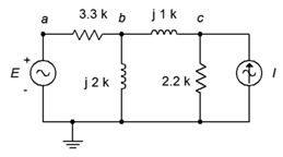
Figure \(\PageIndex{9}\)
18. Use nodal analysis to find the current through the 2.2 k\(\Omega\) resistor in Figure \(\PageIndex{9}\). \(E = 240\angle 0^{\circ}\), \(I = 100E−3\angle 0^{\circ}\).
19. Use nodal analysis to find \(v_{bc}\) in the circuit of Figure \(\PageIndex{10}\).
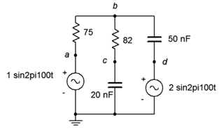
Figure \(\PageIndex{10}\)
20. Use nodal analysis to find the current through the 2.7 k\(\Omega\) resistor in the circuit of Figure \(\PageIndex{11}\).
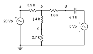
Figure \(\PageIndex{11}\)
21. Given the circuit in Figure \(\PageIndex{12}\), use nodal analysis to determine \(v_{ba}\). \(E_1 = 1\angle 0^{\circ}\), \(E_2 = 2\angle 0^{\circ}\).
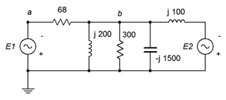
Figure \(\PageIndex{12}\)
22. Given the circuit in Figure \(\PageIndex{13}\), use nodal analysis to determine \(v_{ad}\). \(E_1 = 9\angle 0^{\circ}\), \(E_2 = 5\angle 40^{\circ}\).
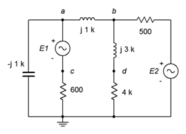
Figure \(\PageIndex{13}\)
23. Use nodal analysis to find \(v_{cb}\) in the circuit of Figure \(\PageIndex{14}\). \(E_1 = 10\angle −180^{\circ}\), \(E_2 = 25\angle 0^{\circ}\).
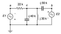
Figure \(\PageIndex{14}\)
24. Given the circuit in Figure \(\PageIndex{15}\), use nodal analysis to determine \(v_{bc}\). \(E = 20\angle 0^{\circ}\), \(R_1\) = 10 k\(\Omega\), \(R_2\) = 30 k\(\Omega\), \(R_3\) = 1 k\(\Omega\), \(X_C = −j15\) k\(\Omega\), \(X_L = j20\) k\(\Omega\).
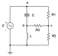
Figure \(\PageIndex{15}\)
25. Given the circuit in Figure \(\PageIndex{16}\), write the mesh loop equations and determine \(v_b\).
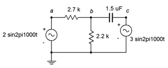
Figure \(\PageIndex{16}\)
26. Use mesh analysis to find the current through the 2.7 k\(\Omega\) resistor in the circuit of Figure \(\PageIndex{16}\).
27. Use mesh analysis to find the current through the 75 \(\Omega\) resistor in the circuit of Figure \(\PageIndex{10}\).
28. Given the circuit in Figure \(\PageIndex{10}\), write the mesh loop equations and determine \(v_c\).
29. Given the circuit in Figure \(\PageIndex{11}\), write the mesh loop equations and determine \(v_b\).
30. Use mesh analysis to find the current through the 1.8 k\(\Omega\) resistor in the circuit of Figure \(\PageIndex{11}\).
31. Use mesh analysis to find the current through the \(j200 \Omega\) inductor in Figure \(\PageIndex{12}\). \(E_1 = 1\angle 0^{\circ}\), \(E_2 = 2\angle 0^{\circ}\).
32. Given the circuit in Figure \(\PageIndex{12}\), write the mesh loop equations and determine \(v_b\). Consider using parallel simplification first. \(E_1 = 36\angle −90^{\circ}\), \(E_2 = 24\angle −90^{\circ}\).
33. Given the circuit in Figure \(\PageIndex{13}\), use mesh analysis to determine \(v_{cd}\). \(E_1 = 0.1\angle 0^{\circ}\), \(E_2 = 0.5\angle 0^{\circ}\).
34. Use mesh analysis to find the current through the 600 \(\Omega\) resistor in the circuit of Figure \(\PageIndex{13}\). \(E_1 = 9\angle 0^{\circ}\), \(E_2 = 5\angle 40^{\circ}\).
35. Use mesh analysis to find the current through the \(−j200 \Omega\) capacitor in the circuit of Figure \(\PageIndex{17}\). \(E_1 = 18\angle 0^{\circ}\), \(E_2 = 12\angle 90^{\circ}\).
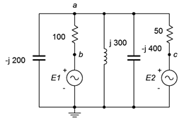
Figure \(\PageIndex{17}\)
36. Given the circuit in Figure \(\PageIndex{17}\), use mesh analysis to determine \(v_{ac}\). \(E_1 = 1\angle 0^{\circ}\), \(E_2 = 500E−3\angle 0^{\circ}\).
37. Given the circuit in Figure \(\PageIndex{14}\), use mesh analysis to determine \(v_c\). \(E_1 = 10\angle −180^{\circ}\), \(E_2 = 25\angle 0^{\circ}\).
38. Use mesh analysis to find the current through the 22 k\(\Omega\) resistor in the circuit of Figure \(\PageIndex{14}\). \(E_1 = 24\angle 0^{\circ}\), \(E_2 = 36\angle 0^{\circ}\).
39. Use mesh analysis to find the current through the \(j300 \Omega\) inductor in Figure \(\PageIndex{18}\). \(E_1 = 1\angle 0^{\circ}\), \(E_2 = 10\angle 90^{\circ}\).
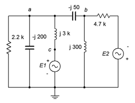
Figure \(\PageIndex{18}\)
40. Given the circuit in Figure \(\PageIndex{18}\), use mesh analysis to determine \(v_a\). \(E_1 = 100\angle 0^{\circ}\), \(E_2 = 90\angle 0^{\circ}\).
41. Given the circuit in Figure \(\PageIndex{15}\), use mesh analysis to determine \(v_{bc}\). \(E = 10\angle 0^{\circ}\), \(R_1\) = 1 k\(\Omega\), \(R_2\) = 2 k\(\Omega\), \(R_3\) = 3 k\(\Omega\), \(X_C = −j4\) k\(\Omega\), \(X_L = j8\) k\(\Omega\).
42. Use mesh analysis to find the current through resistor \(R_3\) in the circuit of Figure \(\PageIndex{15}\). \(E = 20\angle 0^{\circ}\), \(R_1\) = 10 k\(\Omega\), \(R_2\) = 30 k\(\Omega\), \(R_3\) = 1 k\(\Omega\), \(X_C = −j15\) k\(\Omega\), \(X_L = j20\) k\(\Omega\).
43. Use mesh analysis to find the current through resistor \(R_3\) in Figure \(\PageIndex{19}\). \(E = 60\angle 0^{\circ}\), \(R_1\) = 1 k\(\Omega\), \(R_2\) = 2 k\(\Omega\), \(R_3\) = 3 k\(\Omega\), \(X_C = −j10\) k\(\Omega\), \(X_L = j20\) k\(\Omega\).
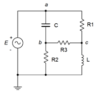
Figure \(\PageIndex{19}\)
44. Given the circuit in Figure \(\PageIndex{19}\), use mesh analysis to determine \(v_{bc}\). \(E = 120\angle 90^{\circ}\), \(R_1\) = 100 k\(\Omega\), \(R_2\) = 20 k\(\Omega\), \(R_3\) = 10 k\(\Omega\), \(X_C = −j5\) k\(\Omega\), \(X_L = j20\) k\(\Omega\).
45. Given the circuit in Figure \(\PageIndex{20}\), use mesh analysis to determine \(v_b\). Consider using source conversion. \(E = 12\angle 0^{\circ}\), \(I = 10E−3\angle 0^{\circ}\).
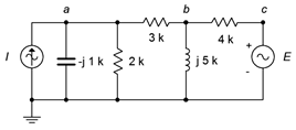
Figure \(\PageIndex{20}\)
46. Use mesh analysis to find the current through the 3 \(\Omega\) resistor in the circuit in Figure \(\PageIndex{20}\). Consider using source conversion. \(E = 15\angle 90^{\circ}\), \(I = 10E−3\angle 0^{\circ}\).
47. Use mesh analysis to find the current through the 2.2 k\(\Omega\) resistor in the circuit in Figure \(\PageIndex{21}\). \(E = 3.3\angle 0^{\circ}\), \(I = 2.1E−3\angle 0^{\circ}\).
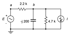
Figure \(\PageIndex{21}\)
48. Given the circuit in Figure \(\PageIndex{21}\), use mesh analysis to determine \(v_b\). \(E = 10\angle 0^{\circ}\), \(I = 30E−3\angle 90^{\circ}\).
49. Given the circuit in Figure \(\PageIndex{22}\), use nodal analysis to determine \(v_{ab}\).
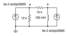
Figure \(\PageIndex{22}\)
50. Use nodal analysis to find the current through the 100 mH inductor in the circuit of Figure \(\PageIndex{22}\).
51. Use nodal analysis to find the current through the 330 \(\Omega\) resistor in the circuit of Figure \(\PageIndex{23}\).
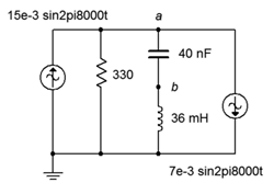
Figure \(\PageIndex{23}\)
52. Given the circuit in Figure \(\PageIndex{23}\), write the node equations and determine \(v_b\).
53. Given the circuit in Figure \(\PageIndex{19}\), use nodal analysis to determine \(v_{bc}\). \(E = 120\angle 0^{\circ}\), \(R_1\) = 1 k\(\Omega\), \(R_2\) = 2 k\(\Omega\), \(R_3\) = 3 k\(\Omega\), \(X_C = −j10\) k\(\Omega\), \(X_L = j20\) k\(\Omega\).
54. Determine the current through the 10 k\(\Omega\) resistor in the circuit of Figure \(\PageIndex{24}\) if \(I_1 = 10E−3\angle −90^{\circ}\).
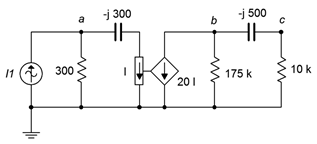
Figure \(\PageIndex{24}\)
55. Determine \(v_b\) in the circuit of Figure \(\PageIndex{24}\) if the source \(I_1 = 20E−3\angle 0^{\circ}\).
56. Determine \(v_c\) in the circuit of Figure \(\PageIndex{25}\) if the source \(E = 3\angle 120^{\circ}\).
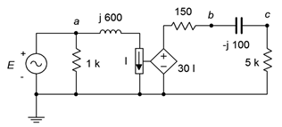
Figure \(\PageIndex{25}\)
57. Determine the current through the 5 k\(\Omega\) resistor in the circuit of Figure \(\PageIndex{25}\) if \(E = 10\angle 0^{\circ}\).
58. In the circuit of Figure \(\PageIndex{26}\), determine the capacitor current if the source \(E = 12\angle 0^{\circ}\).
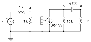
Figure \(\PageIndex{26}\)
59. In the circuit of Figure \(\PageIndex{26}\), determine \(v_c\) if the source \(E = 8\angle 90^{\circ}\).
60. In the circuit of Figure \(\PageIndex{27}\), determine \(v_b\) if the source \(E = 12\angle −90^{\circ}\).
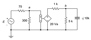
Figure \(\PageIndex{27}\)
61. In the circuit of Figure \(\PageIndex{27}\), determine the current flowing into the 1 k\(\Omega\) resistor if the source \(E = 6\angle 0^{\circ}\).
62. In the circuit of Figure \(\PageIndex{28}\), determine the current flowing into the 600 \(\Omega\) resistor if \(I_1 = 1E−3\angle 180^{\circ}\).
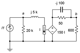
Figure \(\PageIndex{28}\)
63. Determine \(v_a\) and \(v_b\) in the circuit of Figure \(\PageIndex{28}\) if the source \(I_1 = 2E−3\angle 0^{\circ}\).
64. Determine \(v_a\) in the circuit of Figure \(\PageIndex{29}\) if the source \(E = 2\angle 0^{\circ}\).
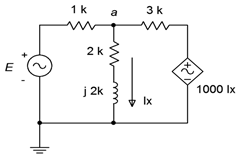
Figure \(\PageIndex{29}\)
65. Given the circuit in Figure \(\PageIndex{29}\), determine the current flowing through the 1 k\(\Omega\) resistor. Assume that \(E = 15\angle 45^{\circ}\).
66. Given the circuit in Figure \(\PageIndex{30}\), determine the current flowing through the 3 k\(\Omega\) resistor if the source \(E = 25\angle 33^{\circ}\).
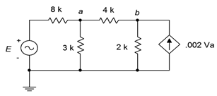
Figure \(\PageIndex{30}\)
67. Given the circuit in Figure \(\PageIndex{30}\), determine \(v_{ab}\). Assume the source \(E = 15\angle −112^{\circ}\).
68. In the circuit of Figure \(\PageIndex{31}\), determine \(v_d\).
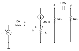
Figure \(\PageIndex{31}\)
69. Given the circuit in Figure \(\PageIndex{31}\), determine the current flowing through the 1 k\(\Omega\) resistor.
70. Given the circuit in Figure \(\PageIndex{32}\), determine the current flowing through the 100 \(\Omega\) resistor.
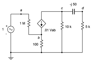
Figure \(\PageIndex{32}\)
71. Determine \(v_d\) in the circuit of Figure \(\PageIndex{32}\).
72. Determine \(v_{ab}\) in the circuit of Figure \(\PageIndex{33}\). \(E = 10\angle 0^{\circ}\)
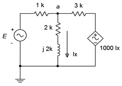
Figure \(\PageIndex{33}\)
Challenge
73. Given the circuit in Figure \(\PageIndex{34}\), write the node equations. \(E_1 = 50\angle 0^{\circ}\), \(E_2 = 35\angle 120^{\circ}\), \(I = 500E−3\angle 90^{\circ}\).
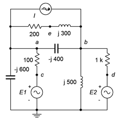
Figure \(\PageIndex{34}\)
74. Given the circuit in Figure \(\PageIndex{34}\), use either mesh or nodal analysis to determine \(v_{ed}\). \(E_1 = 9\angle 0^{\circ}\), \(E_2 = 12\angle 0^{\circ}\), \(I = 50E−3\angle 0^{\circ}\).
75. Given the circuit in Figure \(\PageIndex{35}\), use mesh analysis to determine \(v_{fc}\). \(E_1 = 12\angle 0^{\circ}\), \(E_2 = 48\angle 0^{\circ}\), \(E_3 = 36\angle 70^{\circ}\).
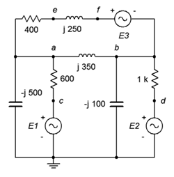
Figure \(\PageIndex{35}\)
76. Find voltage \(v_{bc}\) in the circuit of Figure \(\PageIndex{36}\) using either mesh or nodal analysis. \(E = 100\angle 0^{\circ}\), \(R_1 = R_2 = 2\) k\(\Omega\), \(R_3\) = 3 k\(\Omega\), \(R_4\) = 10 k\(\Omega\), \(R_5\) = 5 k\(\Omega\), \(X_{C1} = X_{C2} = −j2\) k\(\Omega\).
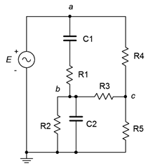
Figure \(\PageIndex{36}\)
77. Given the circuit in Figure \(\PageIndex{37}\), use nodal analysis to find \(v_{ac}\). \(I_1 = 8E−3\angle 0^{\circ}\), \(I_2 = 12E−3\angle 0^{\circ}\), \(E = 50\angle 0^{\circ}\).
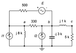
Figure \(\PageIndex{37}\)
78. Given the circuit in Figure \(\PageIndex{38}\), use nodal analysis to determine \(v_{ad}\). \(I_1 = 0.1\angle 0^{\circ}\), \(I_2 = 0.2\angle 0^{\circ}\), \(I_3 = 0.3\angle 0^{\circ}\).
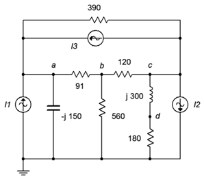
Figure \(\PageIndex{38}\)
79. Given the circuit in Figure \(\PageIndex{39}\), determine \(v_{ad}\). \(E_1 = 15\angle 0^{\circ}\), \(E_2 = 6\angle 0^{\circ}\), \(I = 100E−3\angle 0^{\circ}\).
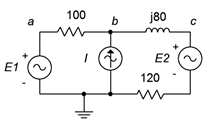
Figure \(\PageIndex{39}\)
80. Given the circuit in Figure \(\PageIndex{40}\), determine \(v_{ad}\). \(E_1 = 22\angle 0^{\circ}\), \(E_2 = −10\angle 0^{\circ}\), \(I = 2E−3\angle 0^{\circ}\).
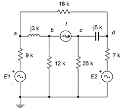
Figure \(\PageIndex{40}\)
81. Given the circuit in Figure \(\PageIndex{41}\), determine \(v_{ab}\). \(I_1 = 1.2\angle 0^{\circ}\), \(I_2 = 2\angle 120^{\circ}\), \(E = 75\angle 0^{\circ}\).
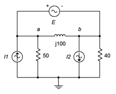
Figure \(\PageIndex{41}\)
82. Given the circuit in Figure \(\PageIndex{42}\), determine \(v_{ad}\). \(I_1 = 0.8\angle 0^{\circ}\), \(I_2 = 0.2\angle 180^{\circ}\), \(I_3 = 0.1\angle 0^{\circ}\), \(E = 15\angle 0^{\circ}\).
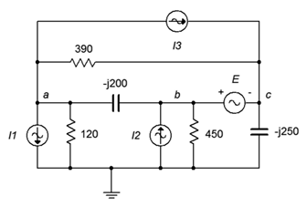
Figure \(\PageIndex{42}\)
Simulation
83. Perform a transient analysis simulation on the circuit of problem 25 (Figure \(\PageIndex{16}\)) to verify the results for \(v_b\).
84. Investigate the variation of \(v_b\) due to frequency in problem 25 (Figure \(\PageIndex{16}\)) by performing an AC simulation. Run the simulation from 10 Hz up to 100 kHz.
85. Investigate the variation of \(v_b\) due to component tolerance in problem 25 (Figure \(\PageIndex{16}\)) by performing a Monte Carlo simulation. Apply a 10% tolerance to the resistors and capacitor.
86. Perform a transient analysis simulation on the circuit of problem 28 (Figure \(\PageIndex{10}\)) to verify the results for \(v_c\).
87. Investigate the variation of \(v_b\) due to frequency in problem 28 (Figure \(\PageIndex{10}\)) by performing an AC simulation. Run the simulation from 1 Hz up to 10 kHz.
88. Investigate the variation of \(v_b\) due to component tolerance in problem 28 (Figure \(\PageIndex{10}\)) by performing a Monte Carlo simulation. Apply a 10% tolerance to the resistors and capacitors.