
6.3: Mesh Analysis
- Page ID
- 25274

\( \newcommand{\vecs}[1]{\overset { \scriptstyle \rightharpoonup} {\mathbf{#1}} } \)
\( \newcommand{\vecd}[1]{\overset{-\!-\!\rightharpoonup}{\vphantom{a}\smash {#1}}} \)
\( \newcommand{\id}{\mathrm{id}}\) \( \newcommand{\Span}{\mathrm{span}}\)
( \newcommand{\kernel}{\mathrm{null}\,}\) \( \newcommand{\range}{\mathrm{range}\,}\)
\( \newcommand{\RealPart}{\mathrm{Re}}\) \( \newcommand{\ImaginaryPart}{\mathrm{Im}}\)
\( \newcommand{\Argument}{\mathrm{Arg}}\) \( \newcommand{\norm}[1]{\| #1 \|}\)
\( \newcommand{\inner}[2]{\langle #1, #2 \rangle}\)
\( \newcommand{\Span}{\mathrm{span}}\)
\( \newcommand{\id}{\mathrm{id}}\)
\( \newcommand{\Span}{\mathrm{span}}\)
\( \newcommand{\kernel}{\mathrm{null}\,}\)
\( \newcommand{\range}{\mathrm{range}\,}\)
\( \newcommand{\RealPart}{\mathrm{Re}}\)
\( \newcommand{\ImaginaryPart}{\mathrm{Im}}\)
\( \newcommand{\Argument}{\mathrm{Arg}}\)
\( \newcommand{\norm}[1]{\| #1 \|}\)
\( \newcommand{\inner}[2]{\langle #1, #2 \rangle}\)
\( \newcommand{\Span}{\mathrm{span}}\) \( \newcommand{\AA}{\unicode[.8,0]{x212B}}\)
\( \newcommand{\vectorA}[1]{\vec{#1}} % arrow\)
\( \newcommand{\vectorAt}[1]{\vec{\text{#1}}} % arrow\)
\( \newcommand{\vectorB}[1]{\overset { \scriptstyle \rightharpoonup} {\mathbf{#1}} } \)
\( \newcommand{\vectorC}[1]{\textbf{#1}} \)
\( \newcommand{\vectorD}[1]{\overrightarrow{#1}} \)
\( \newcommand{\vectorDt}[1]{\overrightarrow{\text{#1}}} \)
\( \newcommand{\vectE}[1]{\overset{-\!-\!\rightharpoonup}{\vphantom{a}\smash{\mathbf {#1}}}} \)
\( \newcommand{\vecs}[1]{\overset { \scriptstyle \rightharpoonup} {\mathbf{#1}} } \)
\( \newcommand{\vecd}[1]{\overset{-\!-\!\rightharpoonup}{\vphantom{a}\smash {#1}}} \)
\(\newcommand{\avec}{\mathbf a}\) \(\newcommand{\bvec}{\mathbf b}\) \(\newcommand{\cvec}{\mathbf c}\) \(\newcommand{\dvec}{\mathbf d}\) \(\newcommand{\dtil}{\widetilde{\mathbf d}}\) \(\newcommand{\evec}{\mathbf e}\) \(\newcommand{\fvec}{\mathbf f}\) \(\newcommand{\nvec}{\mathbf n}\) \(\newcommand{\pvec}{\mathbf p}\) \(\newcommand{\qvec}{\mathbf q}\) \(\newcommand{\svec}{\mathbf s}\) \(\newcommand{\tvec}{\mathbf t}\) \(\newcommand{\uvec}{\mathbf u}\) \(\newcommand{\vvec}{\mathbf v}\) \(\newcommand{\wvec}{\mathbf w}\) \(\newcommand{\xvec}{\mathbf x}\) \(\newcommand{\yvec}{\mathbf y}\) \(\newcommand{\zvec}{\mathbf z}\) \(\newcommand{\rvec}{\mathbf r}\) \(\newcommand{\mvec}{\mathbf m}\) \(\newcommand{\zerovec}{\mathbf 0}\) \(\newcommand{\onevec}{\mathbf 1}\) \(\newcommand{\real}{\mathbb R}\) \(\newcommand{\twovec}[2]{\left[\begin{array}{r}#1 \\ #2 \end{array}\right]}\) \(\newcommand{\ctwovec}[2]{\left[\begin{array}{c}#1 \\ #2 \end{array}\right]}\) \(\newcommand{\threevec}[3]{\left[\begin{array}{r}#1 \\ #2 \\ #3 \end{array}\right]}\) \(\newcommand{\cthreevec}[3]{\left[\begin{array}{c}#1 \\ #2 \\ #3 \end{array}\right]}\) \(\newcommand{\fourvec}[4]{\left[\begin{array}{r}#1 \\ #2 \\ #3 \\ #4 \end{array}\right]}\) \(\newcommand{\cfourvec}[4]{\left[\begin{array}{c}#1 \\ #2 \\ #3 \\ #4 \end{array}\right]}\) \(\newcommand{\fivevec}[5]{\left[\begin{array}{r}#1 \\ #2 \\ #3 \\ #4 \\ #5 \\ \end{array}\right]}\) \(\newcommand{\cfivevec}[5]{\left[\begin{array}{c}#1 \\ #2 \\ #3 \\ #4 \\ #5 \\ \end{array}\right]}\) \(\newcommand{\mattwo}[4]{\left[\begin{array}{rr}#1 \amp #2 \\ #3 \amp #4 \\ \end{array}\right]}\) \(\newcommand{\laspan}[1]{\text{Span}\{#1\}}\) \(\newcommand{\bcal}{\cal B}\) \(\newcommand{\ccal}{\cal C}\) \(\newcommand{\scal}{\cal S}\) \(\newcommand{\wcal}{\cal W}\) \(\newcommand{\ecal}{\cal E}\) \(\newcommand{\coords}[2]{\left\{#1\right\}_{#2}}\) \(\newcommand{\gray}[1]{\color{gray}{#1}}\) \(\newcommand{\lgray}[1]{\color{lightgray}{#1}}\) \(\newcommand{\rank}{\operatorname{rank}}\) \(\newcommand{\row}{\text{Row}}\) \(\newcommand{\col}{\text{Col}}\) \(\renewcommand{\row}{\text{Row}}\) \(\newcommand{\nul}{\text{Nul}}\) \(\newcommand{\var}{\text{Var}}\) \(\newcommand{\corr}{\text{corr}}\) \(\newcommand{\len}[1]{\left|#1\right|}\) \(\newcommand{\bbar}{\overline{\bvec}}\) \(\newcommand{\bhat}{\widehat{\bvec}}\) \(\newcommand{\bperp}{\bvec^\perp}\) \(\newcommand{\xhat}{\widehat{\xvec}}\) \(\newcommand{\vhat}{\widehat{\vvec}}\) \(\newcommand{\uhat}{\widehat{\uvec}}\) \(\newcommand{\what}{\widehat{\wvec}}\) \(\newcommand{\Sighat}{\widehat{\Sigma}}\) \(\newcommand{\lt}{<}\) \(\newcommand{\gt}{>}\) \(\newcommand{\amp}{&}\) \(\definecolor{fillinmathshade}{gray}{0.9}\)Mesh analysis is similar to nodal analysis in that it can handle complex multi-source circuits. In some ways it is the mirror image of nodal analysis. While nodal analysis uses Kirchhoff's current law to create a series of current summations at various nodes, mesh analysis uses Kirchhoff's voltage law to create a series of loop equations that can be solved for mesh currents. The current through any particular component may be a mesh current or a combination of mesh currents. Of course, once those currents are found, it is a short hop to find any desired voltage. Mesh does have one limitation that nodal doesn't: Mesh analysis requires that the circuit be planar. That is, the circuit must be able to be drawn on a flat surface without any wires crossing each other. Another way of looking at it is that planar circuits can be drawn to appear as a series of boxes butting up against each other. To get a visceral idea of this notion, grab a piece of paper and place four dots on it. Try to draw a line from each dot to every other dot but without crossing any lines. After a few tries, you should be successful. Now try it with five dots. You can't do it unless you “draw in the air” and hop over other lines. Obviously, that's possible with real circuits because they're 3D. Therefore there are circuits that cannot be solved using mesh.
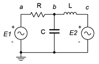
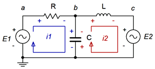
Consider the circuit of Figure \(\PageIndex{1}\). This circuit has two voltage sources and cannot be simplified further, although it can be solved using either superposition or nodal analysis. For mesh analysis, we begin by designating a set of current loops. These loops should be minimal in size and together cover all components at least once. By convention, the loops are drawn with a clockwise reference direction. There is nothing magical about them being clockwise, it is just a matter of consistency. The annotated version of the circuit is redrawn in Figure \(\PageIndex{2}\).
Here we have two loop currents, \(i_1\) and \(i_2\). Note that all components exist in at least one loop (and sometimes in more than one loop, like capacitor \(C\)). Depending on circuit values, one or more of these loop directions may in fact be opposite of reality. This is not a problem. If the true reference direction is opposite, then the currents will show up as negative values, and thus we know that the real reference direction is counterclockwise. Just remember that a positive result means a clockwise direction and negative indicates counterclockwise.
We begin by writing KVL equations for each loop.
Loop 1: \(E_1\) = voltage across \(R\) + voltage across \(X_C\)
Loop 2: \(−E_2\) = voltage across \(X_C\) + voltage across \(X_L\)
Note that \(E_2\) is negative as \(i_2\) is drawn flowing out of its negative terminal. Now expand the voltage terms using Ohm's law. The resistor and inductor each see a single current, \(i_1\) and \(i_2\), respectively. The capacitor experiences both currents. From the perspective of loop 1, \(i_2\) is flowing in the opposite direction. Thus, the net current is \(i_1 − i_2\). From the perspective of loop 2, \(i_1\) is flowing in the opposing direction and thus the net current is \(i_2 − i_1\). The reference voltage polarities reinforce this notion.
Loop 1: \(E_1 = i_1 R + (i_1 − i_2)(−jX_C)\)
Loop 2: \(−E_2 = i_2 (jX_L) + (i_2 − i_1)(−jX_C)\)
Multiplying out and collecting terms yields:
Loop 1: \(E_1 = (R −jX_C) i_1 − (−jX_C) i_2\)
Loop 2: \(−E_2 = − (−jX_C) i_1 + (jX_L −jX_C) i_2\)
As the component values and source voltages are known, we have two equations with two unknowns. These can be solved for \(i_1\) and \(i_2\) using the simultaneous equation solution techniques of your choice.
Example \(\PageIndex{1}\)
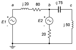
For the circuit of Figure \(\PageIndex{3}\), determine vb and vc. The sources are: \(E_1 = 9\angle 0^{\circ}\) volts and \(E_2 = 12\angle −90^{\circ}\) volts.
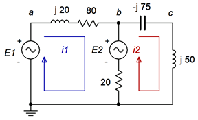
We begin by labeling our loops, as shown in Figure \(\PageIndex{4}\). Each loop will generate an equation based on a KVL summation around that loop. We will number the components from left to right, as usual.
For loop 1:
\[E_1 −E_2 = ( jX_{L1}+R_1 )i_1+R_2 (i_1 −i_2 ) \nonumber \]
\[E_1 −E_2 = (R_1+R_2+jX_{L1})i_1 −R_2 i_2 \nonumber \]
\[9\angle 0^{\circ} V −12\angle −90^{\circ} V = (20+80+j 20 \Omega )i_1 −20\Omega i_2 \nonumber \]
\[15\angle 53.1^{\circ} V = (100+j 20 \Omega )i_1 −20\Omega i_2 \nonumber \]
Repeat for loop 2:
\[E_2 = (− jX_C+jX_{L2})i_2+R_2 (i_2 −i_1 ) \nonumber \]
\[E_2 =−R_2 i_1+(R_2 − jX_C+jX_{L2})i_2 \nonumber \]
\[12\angle −90^{\circ} V = −20\Omega i_1 +(20 − j 75+j 50\Omega )i_2 \nonumber \]
\[12\angle −90^{\circ} V = −20\Omega i_1 +(20 − j 25\Omega )i_2 \nonumber \]
The two loop equations are:
\[15\angle 53.1^{\circ} V = (100+j 20\Omega )i_1 −20\Omega i_2 \nonumber \]
\[12\angle −90^{\circ} V = −20\Omega i_1 +(20− j 25\Omega )i_2 \nonumber \]
The equations show diagonal symmetry. The currents are \(i_1 = 0.1785\angle 19.9^{\circ}\) amps and \(i_2 = 0.3529\angle −21.4^{\circ}\) amps. To find the voltages \(v_b\) and \(v_c\), we just need to apply Ohm's law. The voltage \(v_c\) is the potential across the \(j50 \Omega\) inductor.
\[v_c = i_2\times jX_{L2} \nonumber \]
\[v_c = 0.3529\angle −21.4^{\circ} A\times j 50\Omega \nonumber \]
\[v_c = 17.64\angle 68.6^{\circ} V \nonumber \]
The potential \(v_b\) is found similarly.
\[v_b = i_2\times (− jX_C+jX_{L2}) \nonumber \]
\[v_b = 0.3529\angle −21.4^{\circ} \times (− j 75\Omega +j 50 \Omega ) \nonumber \]
\[v_b = 8.823\angle −111.4^{\circ} V \nonumber \]
For verification, we can also find \(v_b\) by subtracting the voltage developed across the series inductor/resistor pair from the first source.
\[v_b = E_1 − i_1\times (R_1+jX_{L1}) \nonumber \]
\[v_b = 9\angle 0^{\circ} V − 0.1785\angle 19.9^{\circ} A\times (80 +j 20 \Omega ) \nonumber \]
\[v_b=8.823\angle −111.4^{\circ} V \nonumber \]
Example \(\PageIndex{2}\)
In the circuit of Figure \(\PageIndex{5}\), find \(v_b\). \(E = 10\angle 0^{\circ}\) volts peak at a frequency of 10 kHz.
The circuit is a bridge network. Even though it has only a single voltage source, basic series-parallel techniques will not work here. Nodal analysis can also work here as can delta-Y conversion, however, mesh is an excellent choice for this layout.

We start by finding the reactance values. Using the standard reactance formulas we find that \(X_L = j628.3 \Omega\) and \(X_C = −j318.3 \Omega\). After substituting these into the original circuit and defining the loops, we have Figure \(\PageIndex{6}\).
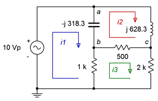
We have three loops with three unknown currents, and therefore three equations. We'll number the resistors from left to right. For loop 1:
\[E = v_C+v_{R1} \nonumber \]
\[E =− jX_C (i_1 −i_2 )+R_1 (i_1 −i_3 ) \nonumber \]
\[E = (R_1 − jX_C )i_1 −(− jX_C )i_2 −R_1 i_3 \nonumber \]
\[10\angle 0^{\circ} V = (1k \Omega − j 318.3\Omega )i_1+j318.3 \Omega i_2 −1k \Omega i_3 \nonumber \]
For loop 2:
\[0 = v_C+v_L+v_{R2} \nonumber \]
\[0 =− jX_C (i_2 −i_1 )+jX_L (i_2 −i_3 )+jX_L i_3 \nonumber \]
\[0 =−(− jX_C )i_1+(R_2+X_L − jX_C )i_2 −R_2 i_3 \nonumber \]
\[0 =−(− j 318.3\Omega )i_1+(500+j 628.3 − j 318.3\Omega )i_2 −500\Omega i_3 \nonumber \]
\[0 = j 318.3\Omega i_1+(500+j 310\Omega )i_2 −500\Omega i_3 \nonumber \]
For loop 3:
\[0 = v_{R1} + v_{R2} + v_{R3} \nonumber \]
\[0 = R_1 (i_3 −i_1 )+R_2 (i_3 −i_2 )+R_3 i_3 \nonumber \]
\[0 =−R_1 i_1 −R_2 i_2+(R_1+R_2+R_3 )i_3 \nonumber \]
\[0 =−1 k\Omega i_1 −500 \Omega i_2+(1k \Omega +500\Omega +2k \Omega )i_3 \nonumber \]
\[0 =−1 k\Omega i_1 −500 \Omega i_2+3.5k \Omega i_3 \nonumber \]
The final set of equations is:
\[10\angle 0^{\circ} V = (1k \Omega − j 318.3\Omega )i_1+j 318.3 \Omega i_2 −1k \Omega i_3 \nonumber \]
\[0 = j 318.3\Omega i_1+(500+j 310 \Omega )i_2 −500\Omega i_3 \nonumber \]
\[0 =−1 k\Omega i_1 −500 \Omega i_2+3.5k \Omega i_3 \nonumber \]
The system of equations has diagonal symmetry. The results are: \(i_1 = 10.24E-3\angle 16^{\circ}\) amps, \(i_2 = 6.754E-3\angle −85.7^{\circ}\) amps and \(i_3 = 2.888E-3\angle −3.13^{\circ}\) amps.
For \(v_b\), this is just the voltage across the 1 k\(\Omega \) resistor. Note that a pair of meshing currents (\(i_1\) and \(i_3\)) are flowing through that resistor, so we must determine the net value of current. If we assume the reference polarity for \(v_b\) is positive, that coincides with the direction of \(i_1\), and thus the net current must be \(i_1 − i_3\). The result is \(i_{net} = 7.57E−3\angle 23.2^{\circ}\) amps. Therefore, \(v_b = 7.57\angle 23.2^{\circ}\) volts.
Computer Simulation
Figure \(\PageIndex{7}\) shows the bridge circuit of Example \(\PageIndex{2}\) captured in a simulator. This will be used to verify the computed result.
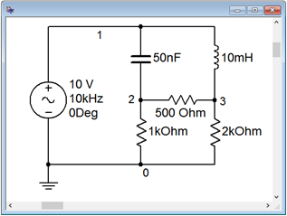
A transient analysis is run on the circuit, plotting node 2 which corresponds to \(v_b\), and node 1, the input voltage, which is handy for phase reference.
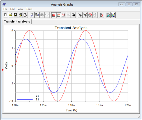
Examining the plot, we can see that the node 2 voltage is just above 7.5 volts peak, as calculated. Further, this waveform leads the the input waveform by just over a quarter of a division. As this plot shows four divisions per cycle, each division is 90 degrees. This indicates a leading or positive phase shift in the low 20 degree range, and that corroborates nicely the computed value of 23.2 degrees.
Inspection Method
Like nodal analysis, it is possible that the system of equations can be obtained directly through inspection. This is true only if the circuit contains no current sources. Look at the final set of equations derived in Example \(\PageIndex{2}\) from Figure \(\PageIndex{6}\). A clear pattern will emerge. To generate an equation for a given loop, simply focus on that loop and ask the following questions: What is the total source voltage in this loop? This yields the voltage constant on the left side of the equals sign. Next, sum the resistance and reactance values in the loop under inspection. This yields the coefficient for that current term. For the other current coefficients, sum the resistances and reactances that are in common between the loop under inspection and the other loops (e.g., for loop 1, \(X_C\) is in common with loop 2). These values will always be negative (an exception arises with a “double negative”, as seen with the capacitor). As usual, the set of equations produced must exhibit diagonal symmetry.
While it is possible to extend this technique to include current sources, usually it is easier and less error-prone to convert the current sources into voltage sources. Then the process can continue with the direct inspection method outlined above. Finally, it is important to remember that the number of loops determines the number of equations to be solved. This method will be illustrated in the example following.
Example \(\PageIndex{3}\)
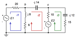
For the circuit of Figure \(\PageIndex{9}\), find \(v_b\) and the current through the 15 \(\Omega \) resistor. \(E_1 = 10\angle 0^{\circ}\) volts peak and \(E_2 = 20\angle 90^{\circ}\) volts peak.
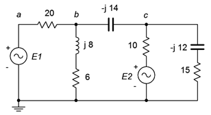
We identify and label three loops, as shown in Figure \(\PageIndex{10}\). This circuit utilizes only voltage sources and no current sources. Therefore, we can apply the inspection method without extra effort.
We start at loop 1 and sum all of the voltage sources. The sole source is \(E_1\).
\[10\angle 0^{\circ} V = \dots \nonumber \]
Now we sum all of the resistances and reactances in this loop. This is the coefficient for the first current term.
\[10\angle 0^{\circ} V =(20\Omega +6\Omega +j 8\Omega )i_1 \dots \nonumber \]
We continue the process by determining the components that are in common between this loop and the next loop. Remember, this coefficient is negative.
\[10\angle 0^{\circ} V =(20\Omega +6\Omega +j 8\Omega )i_1 −(6\Omega +j 8\Omega )i_2 \dots \nonumber \]
We repeat the process by determining the common components with the next loop. This coefficient is negative. In this situation, no components are in common between loops 1 and 3. We shall leave in placeholder with a coefficient of zero, just as a reminder that we didn't forget anything and also to ensure that the coefficients in the final set of equations line up nicely.
\[10\angle 0^{\circ} V = (26+j 8\Omega )i_1 −(6+j 8\Omega )i_2 −0i_3 \nonumber \]
We now move to loop 2 and repeat the sequence of steps. There is only one source, \(E_2\), and it shows up negative as mesh current \(i_2\) is flowing out of its negative terminal. The result is:
\[−20\angle 90^{\circ} V =−(6+j 8\Omega )i_1+(6+10+j8 − j 14 \Omega )i_2 −10\Omega i_3 \nonumber \]
\[−20\angle 90^{\circ} V =−(6+j 8\Omega )i_1+(16 − j 6\Omega )i_2 −10\Omega i_3 \nonumber \]
And finally the third loop. Here the second source shows up as positive.
\[20 \angle 90^{\circ} V =−0i_1−10\Omega i_2 −(10+15− j 12\Omega )i_3 \nonumber \]
\[20 \angle 90^{\circ} V =−0i_1−10\Omega i_2 −(25− j 12\Omega )i_3 \nonumber \]
The completed system of equations is:
\[10\angle 0^{\circ} V = (26+j 8\Omega )i_1 −(6+j8\Omega )i_2 −0i_3 \nonumber \]
\[−20\angle 90^{\circ} V =−(6+j 8\Omega )i_1+(16 − j 6\Omega )i_2 −10\Omega i_3 \nonumber \]
\[20 \angle 90^{\circ} V =−0i_1−10\Omega i_2 −(25 − j 12\Omega )i_3 \nonumber \]
The system has diagonal symmetry. The resulting currents are: \(i_1 = 0.6131\angle −15.5^{\circ}\) amps, \(i_2 = 0.6687\angle −49.2^{\circ}\) amps and \(i_3 = 0.5611\angle 99.3^{\circ}\) amps.
The current through the 15 \(\Omega \) resistor is \(i_3\), so that much is done. Regarding \(v_b\), it can be found using Ohm's law as \(v_b\) is the series connection of the 6 \(\Omega \) resistor and \(j8 \Omega\) inductor times the current through them. This current is the pair of meshing currents \(i_1\) and \(i_2\). Assuming the reference polarity for \(v_b\) is positive, that is the direction of \(i_1\), and thus the net current must be \(i_1 − i_2\). The result is \(0.375\angle 65.8^{\circ}\) amps. Therefore, \(v_b = 3.75\angle 119^{\circ}\) volts. To crosscheck this, we can subtract the voltage across the 20 \(\Omega \) resistor from \(E_1\). That's \(10\angle 0^{\circ}\) volts minus 20 \(\Omega \) times \(0.6131\angle −15.5^{\circ}\) amps, or \(3.75\angle 119^{\circ}\) volts, as expected.
Supermesh
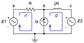
On occasion you may find a current source which has no associated internal impedance, such as the one in the circuit of Figure \(\PageIndex{11}\). This is similar to the situation discussed previously with nodal analysis where a voltage source does not have a specified internal impedance. As with nodal, there are two ways of solving this predicament. The first technique is to add a very large impedance in parallel with the current source and then perform a source conversion on the pair so that the inspection method of mesh can be used. The larger the value of this impedance, the greater the accuracy. As a general rule it should be at least a couple of orders of magnitude larger than any surrounding impedance, and preferably larger. The second technique is to use supermesh. A supermesh is a larger mesh loop than contains other mesh loops inside of it.
Refer to the circuit shown in Figure \(\PageIndex{11}\). In the center we have a current source, \(I_s\), which lacks an associated internal impedance. Two traditional mesh loops, \(i_1\) and \(i_2\), are labeled as usual. The problem here is that we cannot use an Ohm's law-based \(i_Z\) voltage drop for \(v_b\). We have no way to express this as the voltage across \(I_s\) is an unknown. On the other hand, what we do know is that Is must equal the combination of the original mesh currents \(i_1\) and \(i_2\). That is, from the perspective of the first loop, \(I_s = i_2 − i_1\). Remember, one or both of the mesh currents could be negative, and thus rotating counterclockwise.
At this point we invoke the idea of a supermesh loop. First, we replace the problematic current source with its ideal internal impedance, an open. Second, a supermesh loop is drawn which encompasses the original two loops. This is shown in Figure \(\PageIndex{12}\). The supermesh loop is shown in red and labeled.
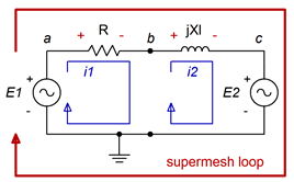
We now perform a KVL summation around the supermesh loop, similar to what we have done in prior work. The difference this time around is that we need to recognize that components each see one of the original mesh currents; namely \(i_1\) or \(i_2\) here. We do not solve for a supermesh current. Instead, we just use the supermesh loop to define the KVL summation. The summation follows:
\[\sum v_{rises} = \sum v_{drops} \nonumber \]
\[E_1 = v_R+v_{XL}+E_2 \nonumber \]
The voltage drops across the resistor and inductor can be expanded using Ohm's law, using the original mesh current associated with each component.
\[E_1 −E_2 = i_1 R +i_2 jX_L \nonumber \]
Also, by inspection,
\[I_s = i_2 −i_1 \text{ or} \nonumber \]
\[i_2 = i_1 +I_s \nonumber \]
We now have two equations with two unknowns and can solve for \(i_1\) and \(i_2\). This procedure is illustrated in the following example.
Example \(\PageIndex{4}\)
Find \(v_b\) for the circuit of Figure \(\PageIndex{13}\). \(E_1 = 20\angle 0^{\circ}\) volts, \(E_1 = 18\angle 90^{\circ}\) volts and \(I_S = 10E−3\angle 0^{\circ}\) amps.
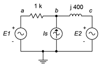
First, we label the loops, as shown in Figure \(\PageIndex{14}\).
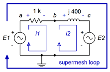
Now we perform a KVL summation around the supermesh loop.
\[\sum v_{rises} = \sum v_{drops} \nonumber \]
\[20 \angle 0^{\circ} V = v_R+v_{XL}+18\angle 90^{\circ} V \nonumber \]
Expand using Ohm's law and rearrange:
\[20 \angle 0^{\circ} V −18\angle 90^{\circ} V = 1k\Omega i_1+j 400 \Omega i_2 \nonumber \]
\[26.9 \angle −42^{\circ} V = 1k\Omega i_1+j 400 \Omega i_2 \nonumber \]
By inspection we can see that:
\[10E-3\angle 0^{\circ} A = i_2 −i_1 \text{ or} \nonumber \]
\[i_2 = i_1 +10E-3\angle 0^{\circ} A \nonumber \]
We can substitute this expression into the prior supermesh expression and solve for \(i_1\):
\[26.9 \angle −42^{\circ} V = 1k\Omega i_1 +j 400 \Omega i_2 \nonumber \]
\[26.9 \angle −42^{\circ} V = 1k\Omega i_1+j 400 \Omega (i_1+10E-3 \angle 0^{\circ} A) \nonumber \]
\[26.9 \angle −42^{\circ} V = 1k\Omega i_1+j 400 \Omega i_1+4\angle 90^{\circ} V \nonumber \]
\[29.7\angle −44.7^{\circ} V = (1 k+j 400\Omega )i_1 \nonumber \]
\[i_1 \approx 27.6E-3\angle −69.5^{\circ} A \nonumber \]
Thus, \(i_2 = 27.6E−3\angle −69.5^{\circ}\) amps + \(10E−3\angle 0^{\circ}\) amps, or \(32.5E−3\angle -52.8^{\circ}\) amps. To determine \(v_b\) we simply subtract the drop across the 1 k\(\Omega\) resistor from \(E_1\):
\[v_b = 20 \angle 0^{\circ} V − i_1 1k \Omega \nonumber \]
\[v_b = 20 \angle 0^{\circ} V − 27.6E-3\angle −69.5^{\circ} A1 k\Omega \nonumber \]
\[v_b \approx 27.85\angle 68.2^{\circ} V \nonumber \]
As a crosscheck, we could also add the voltage across the inductor to \(E_2\):
\[v_b = 18\angle 90^{\circ} V +i_2 j 400\Omega \nonumber \]
\[v_b = 18\angle 90^{\circ} V +32.5E-3\angle −52.8^{\circ} A j400 \Omega \nonumber \]
\[v_b \approx 27.85\angle 68.2^{\circ} V \nonumber \]
Comparison of Nodal and Mesh
Having covered both nodal and mesh in some detail, it is fair to look at the two techniques to gauge their strengths and weaknesses. Compared to nodal analysis, mesh analysis has the advantage of dealing with impedances rather than admittances when writing the system of equations. Further, the mesh inspection method works with voltage sources, which tends to be convenient for many circuits, while the nodal inspection method requires current sources. On the down side, the resulting set of mesh currents requires further processing in order to find either branch currents or node voltages. In contrast, nodal analysis produces node voltages directly with no further processing. Mesh also has the disadvantage of being limited to planar circuits while there is no such limit to nodal. Ultimately, instead of thinking in terms of which technique is “better” overall, it is more efficient to use the proper tool for the job at hand. For example, if a circuit is populated with voltage sources, mesh might be the more efficient route, especially if specific currents are desired. On the other hand, if you need to find voltages in a circuit that contains numerous current sources, nodal would be more effective.