1.1: RF and Microwave Engineering

Radio communications is the main driver of RF system development, leading to RF technology evolution at an unprecedented pace. A radio signal is a signal that is coherently generated, radiated by a transmit antenna, propagated through the air, collected by a receive antenna, and then amplified and information extracted. The radio spectrum is part of the electromagnetic (EM) spectrum exploited by humans for communications. A broad categorization of the EM spectrum is shown in Table \(\PageIndex{1}\). Today radios operate from \(3\text{ Hz}\) (for submarine communications) to \(300\text{ GHz}\) (proposed for 6G cellular communications).

Name or band	Frequency	Wavelength
Radio frequency	\(3\text{ Hz} - 300\text{ GHz}\)	\(100,000\text{ km} - 1\text{ mm}\)
Microwave	\(300\text{ MHz} - 300\text{ GHz}\)	\(1\text{ m} - 1\text{ mm}\)
Millimeter (\(\text{mm}\)) band	\(110-300\text{ GHz}\)	\(2.7\text{mm} - 1.0\text{ mm}\)
Infrared	\(300\text{ GHz} - 400\text{ THz}\)	\(1\text{ mm} - 750\text{ nm}\)
Far infrared	\(300\text{ GHz} - 20\text{ THz}\)	\(1\text{ mm} - 15\:\mu\text{m}\)
Long-wavelength infrared	\(20\text{ THz} - 37.5\text{ THz}\)	\(15 - 8\:\mu\text{m}\)
Mid-wavelength infrared	\(37.5 - 100\text{ THz}\)	\(8- 3\:\mu\text{m}\)
Short-wavelength infrared	\(100\text{ THz} - 214\text{ THz}\)	\(3 - 1.4\:\mu\text{m}\)
Near infrared	\(214\text{ THz} - 400\text{ THz}\)	\(1.4\:\mu\text{m} - 750\text{ nm}\)
Visible	\(400\text{ THz} - 750\text{ THz}\)	\(750 - 400\text{ mm}\)
Ultravoilet	\(750\text{ THz} - 30\text{ PHz}\)	\(400 - 10\text{ nm}\)
X-Ray	\(30\text{ PHz} - 30\text{ EHz}\)	\(10- 0.01\text{ nm}\)
Gamma Ray	\(> 15\text{ EHz}\)	\(< 0.02\text{ nm}\)
Gigahertz, \(\text{GHz} = 109\text{ Hz}\); terahertz, \(\text{THz} = 1012\text{ Hz}\); pentahertz, \(\text{PHz} = 1015\text{ Hz}\); exahertz, \(\text{EHz} = 1018\text{ Hz}\).

Table \(\PageIndex{1}\): Broad electromagnetic spectrum divisions.

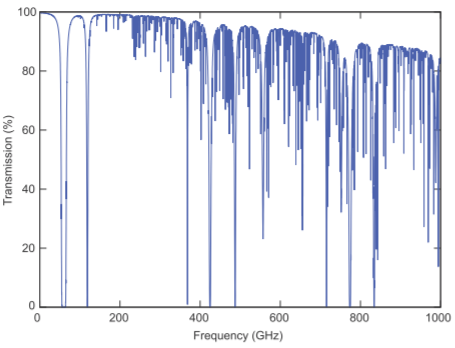
Figure \(\PageIndex{1}\): : Atmospheric transmission at Mauna Kea, with a height of \(4.2\text{ km}\), on the Island of Hawaii where the atmospheric pressure is \(60\%\) of that at sea level and the air is dry with a precipitable water vapor level of \(0.001\text{ mm}\). After [1].

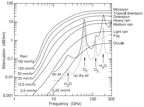
Figure \(\PageIndex{2}\): Excess attenuation due to atmospheric conditions showing the effect of rain on RF transmission at sea level. Curve (a) is atmospheric attenuation, due to excitation of molecular resonances, of very dry air at \(0^{\circ}\text{C}\), curve (b) is for typical air (i.e. less dry) at \(20^{\circ}\text{C}\). The attenuation shown for fog and rain is additional (in \(\text{dB}\)) to the atmospheric absorption shown as curve (b).

Propagating RF signals in air are absorbed by molecules in the atmosphere primarily by molecular resonances such as the bending and stretching of bonds which converts EM energy into heat. The transmittance of radio signals versus frequency in dry air at an altitude of \(4.2\text{ km}\) is shown in Figure \(\PageIndex{1}\) and there are many transmission holes due to molecular resonances. The lowest frequency molecular resonance in dry air is the oxygen resonance centered at \(60\text{ GHz}\), but below that the absorption in dry air is very small. Attenuation increases with higher water vapor pressure peaking at \(22\text{ GHz}\) and broadening due to the close packing of molecules in air. The effect of water is seen in Figure \(\PageIndex{2}\) and it is seen that rain and water vapor have little effect on cellular communications which are below \(5\text{ GHz}\) except for millimeter-wave 5G.

RF signals diffract and so can bend around structures and penetrate into valleys. The ability to diffract reduces with increasing frequency. However, as frequency increases the size of antennas decreases and the capacity to carry information increases. A very good compromise for mobile communications is at UHF, \(300\text{ MHz}\) to \(4\text{ GHz}\), where antennas are of convenient size and there is a good ability to diffract around objects and even penetrate walls.

1.1.1 Electromagnetic Fields

Communicating using EM signals built from an understanding of magnetic induction based on the experiments of Faraday in 1831 [2] in which he investigated the relationship of magnetic fields and currents, and now known as Faraday’s law. This and the other static field laws are not enough to describe radio waves. The required description is embodied in Maxwell’s equations and after these were developed it took little time before radio was invented.

1.1.2 Static Field Laws

There are two components of the EM field, the electric field, \(E\), with units of volts per meter (\(\text{V/m}\)), and the magnetic field, \(H\), with units of amperes per meter (\(\text{A/m}\)). There are also two flux quantities with the first being \(D\), the electric flux density, with units of coulombs per square meter (\(\text{C/m}^{2}\)), and the other is \(B\), the magnetic flux density, with units of teslas (\(\text{T}\)). \(B\) and \(H\), and \(D\) and \(E\), are related to each other by the properties of the medium, which are embodied in the quantities \(\mu\) and \(\varepsilon\) (with the caligraphic letter, e.g. \(\mathcal{B}\), denoting a time domain quantity):

\[\label{eq:1}\overline{\mathcal{B}}=\mu\overline{\mathcal{H}} \]

\[\label{eq:2}\overline{\mathcal{D}}=\varepsilon\overline{\mathcal{E}} \]

where the over bar denotes a vector quantity, and \(\mu\) is the permeability of the medium and describes the ability to store magnetic energy in a region. The permeability in free space (or vacuum) is \(\mu_{0}=4\pi\times 10^{-7}\text{ H/m}\) and then

\[\label{eq:3}\overline{\mathcal{B}}=\mu_{0}\overline{\mathcal{H}} \]

The other material quantity is the permittivity, \(\varepsilon\), and in a vacuum

\[\label{eq:4}\overline{\mathcal{D}}=\varepsilon_{0}\overline{\mathcal{E}} \]

where \(\varepsilon_{0} = 8.854\times 10^{-12}\text{ F/m}\) is the permittivity of a vacuum. The relative permittivity, \(\varepsilon_{r}\), the relative permeability, \(\mu_{r}\), are defined as

\[\label{eq:5}\varepsilon_{r}=\varepsilon /\varepsilon_{0}\qquad\text{and}\qquad\mu_{r}=\mu /\mu_{0} \]

Biot-Savart Law

The Biot–Savart law relates current to magnetic field as, see Figure 1-3,

\[\label{eq:6}d\overline{H} = \frac{Id\ell\times\hat{a}_{R}}{4\pi R^{2}} \]

with units of amperes per meter in the SI system. In Equation \(\eqref{eq:6}\) \(d\overline{H}\) is the incremental static \(H\) field, \(I\) is current, \(d\ell\) is the vector of the length of a filament of current \(I\), \(\hat{a}_{R}\) is the unit vector in the direction from the current filament to the magnetic field, and \(R\) is the distance between the filament and the magnetic field. The \(d\overline{H}\) field is directed at right angles to \(\hat{a}_{R}\) and the current filament. So Equation \(\eqref{eq:6}\) says that a filament of current produces a

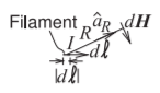
Figure \(\PageIndex{3}\): Diagram illustrating the Biot-Savart law. The law relates a static filament of current to the incremental \(H\) field at a distance.

Figure \(\PageIndex{4}\): Diagram illustrating Faraday’s law. The contour \(\ell\) encloses the surface.

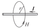
Figure \(\PageIndex{5}\): Diagram illustrating Ampere’s law. Ampere’s law relates the current, \(I\), on a wire to the magnetic field around it, \(H\).

magnetic field at a point. The total magnetic field from a current on a wire or surface can be found by modeling the wire or surface as a number of current filaments, and the total magnetic field at a point is obtained by integrating the contributions from each filament.

Faraday's Law of Induction

Faraday’s law relates a time-varying magnetic field to an induced voltage drop, \(V\), around a closed path, which is now understood to be \(\oint_{\ell}\overline{\mathcal{E}}\cdot d\ell\), that is, the closed contour integral of the electric field,

\[\label{eq:7}V=\oint_{\ell}\overline{\mathcal{E}}\cdot d\ell = -\oint_{s}\frac{\partial\overline{\mathcal{B}}}{\partial t}\cdot d\text{s} \]

and this has the units of volts in the SI unit system. The operation described in Equation \(\eqref{eq:7}\) is illustrated in Figure \(\PageIndex{4}\).

Ampere's Circuital Law

Ampere’s circuital law, often called just Ampere’s law, relates direct current and the static magnetic field \(\overline{\mathcal{H}}\), see Figure \(\PageIndex{5}\):

\[\label{eq:8}\oint_{\ell}\overline{H}\cdot d\ell = I_{\text{enclosed}} \]

That is, the integral of the magnetic field around a loop is equal to the current enclosed by the loop. Using symmetry, the magnitude of the magnetic field at a distance \(r\) from the center of the wire shown in Figure \(\PageIndex{5}\) is

\[\label{eq:9}H=|I|/(2\pi r) \]

Gauss's Law

The final static EM law is Gauss’s law, which relates the static electric flux density vector, \(\overline{D}\), to charge. With reference to Figure \(\PageIndex{6}\), Gauss’s law in integral form is

\[\label{eq:10}\oint_{s}\overline{D}\cdot d\text{s}=\int_{v}\rho_{v}\cdot dv=Q_{\text{enclosed}} \]

This states that the integral of the constant electric flux vector, \(\overline{D}\), over a closed surface is equal to the total charge enclosed by the surface, \(Q_{\text{enclosed}}\).

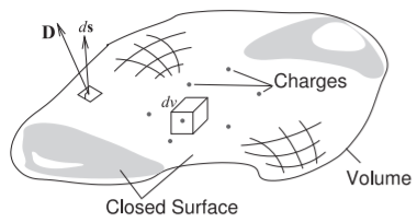
Figure \(\PageIndex{6}\): Diagram illustrating Gauss’s law. Charges are distributed in the volume enclosed by the closed surface. An incremental area is described by the vector \(d\text{s}\), which is normal to the surface and whose magnitude is the area of the incremental area.

Gauss's Law of Magnetism

Gauss’s law of magnetism parallels Gauss’s law which applies to electric fields and charges. In integral form the law is

\[\label{eq:11}\oint_{s}\overline{B}\cdot d\text{s}=0 \]

This states that the integral of the constant magnetic flux vector, \(\overline{D}\), over a closed surface is zero reflecting the fact that magnetic charges do not exist.

1.1.3 Maxwell's Equations

The essential step in the invention of radio was the development of Maxwell’s equations in 1861. Before Maxwell’s equations were postulated, several static EM laws were known. Taken together they cannot describe the propagation of EM signals, but they can be derived from Maxwell’s equations. Maxwell’s equations cannot be derived from the static electric and magnetic field laws. Maxwell’s equations embody additional insight relating spatial derivatives to time derivatives, which leads to a description of propagating fields. Maxwell’s equations are

\[\label{eq:12}\nabla\times\overline{\mathcal{E}}=-\frac{\partial\overline{\mathcal{B}}}{\partial t}-\overline{\mathcal{M}} \]

\[\label{eq:13}\nabla\cdot\overline{\mathcal{D}}=\rho_{V} \]

\[\label{eq:14}\nabla\times\overline{\mathcal{H}}=\frac{\partial\overline{\mathcal{D}}}{\partial t}+ \overline{\mathcal{J}} \]

\[\label{eq:15}\nabla\cdot\overline{\mathcal{B}}=\rho_{mV} \]

The additional quantities in Equations \(\eqref{eq:12}\)-\(\eqref{eq:15}\) are

• \(\overline{\mathcal{J}}\), the electric current density, with units of amperes per square meter (\(\text{A/m}^{2}\));
• \(\rho_{V}\), the electric charge density, with units of coulombs per cubic meter (\(\text{C/m}^{3}\));
• \(\rho_{mV}\), the magnetic charge density, with units of webers per cubic meter (\(\text{Wb/m}^{3}\)); and
• \(\overline{\mathcal{M}}\), the magnetic current density, with units of volts per square meter (\(\text{V/m}^{2}\)).

Magnetic charges do not exist, but their introduction through the magnetic charge density, \(\rho _{mV}\), and the magnetic current density, \(\overline{\mathcal{M}}\), introduce an aesthetically appealing symmetry to Maxwell’s equations. Maxwell’s equations are differential equations, and as with most differential equations, their solution is obtained with particular boundary conditions, which in radio engineering are imposed by conductors.

Maxwell’s equations have three types of derivatives. First, there is the time derivative, \(\partial /\partial t\). Then there are two spatial derivatives, \(\nabla\times\), called curl, capturing the way a field circulates spatially (or the amount that it curls up on itself), and \(\nabla\cdot\), called the div operator, describing the spreading-out of a

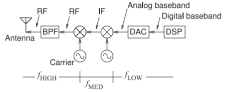
Figure \(\PageIndex{7}\): A simple transmitter with low, \(f_{\text{LOW}}\), medium, \(f_{\text{MED}}\), and high frequency, \(f_{\text{HIGH}}\), sections. The mixers can be idealized as multipliers that boost the frequency of the input baseband or IF signal by the frequency of the carrier.

field. In rectangular coordinates, curl, \(\nabla\times\), describes how much a field circles around the \(x,\: y,\) and \(z\) axes. That is, the curl describes how a field circulates on itself. So Equation \(\eqref{eq:12}\) relates the amount an electric field circulates on itself to changes of the \(B\) field in time. So a spatial derivative of electric fields is related to a time derivative of the magnetic field. Also in Equation \(\eqref{eq:14}\) the spatial derivative of the magnetic field is related to the time derivative of the electric field. These are the key elements that result in self-sustaining propagation.

Div, \(\nabla\cdot\), describes how a field spreads out from a point. How fast a field varies with time, \(\partial\overline{\mathcal{B}}/\partial t\) and \(\partial\overline{\mathcal{D}}/\partial t\), depends on frequency. The more interesting derivatives are \(\nabla\times\overline{\mathcal{E}}\) and \(\nabla\times\overline{\mathcal{H}}\) which describe how fast a field can change spatially—this depends on wavelength relative to geometry. If the cross-sectional dimensions of a transmission line are less than a wavelength (\(\lambda /2\) or \(\lambda /4\) in different circumstances when there are conductors), then it will be impossible for the fields to curl up on themselves and so there will be only one solution (with no or minimal variation of the \(E\) and \(H\) fields) or, in some cases, no solution to Maxwell’s equations.