1.3: RF Power Calculations

1.3.1 RF Propagation

As an RF signal propagates away from a transmitter the power density reduces conserving the power in the EM wave. In the absence of obstacles and without atmospheric attenuation the total power passing through the surface of a sphere centered on a transmitter is equal to the power transmitted. Since the area of the sphere of radius \(r\) is \(4\pi r^{2}\), the power density, e.g. in \(\text{W/m}^{2}\), at a distance \(r\) drops off as \(1/r^{2}\). With obstacles the EM wave can be further attenuated.

Example \(\PageIndex{1}\): Signal Propagation

A signal is received at a distance \(r\) from a transmitter and the received power drops off as \(1/r^{2}\). When \(r = 1\text{ km}\), \(100\text{ nW}\) is received. What is \(r\) when the received power is \(100\text{ fW}\)?

Solution

The signal collected by the receiver is proportional to the power density of the EM signal. The received signal power \(P_{r} = k/r^{2}\) where \(k\) is a constant. This leads to

\[\label{eq:1}\frac{P_{r}(1\text{ km})}{P_{r}(r)}=\frac{100\text{ nW}}{100\text{ fW}}=10^{6}=\frac{kr^{2}}{k(1\text{ km})^{2}}=\frac{r^{2}}{(10^{3}\text{ m})^{2}};\quad r=\sqrt{10^{12}\text{ m}^{2}}=1000\text{ km} \]

1.3.2 Logarithm

A cellular phone can reliably receive a signal as small as \(100\text{ fW}\) and the signal to be transmitted could be \(1\text{ W}\). So the same circuitry can encounter signals differing in power by a factor of \(10^{13}\). To handle such a large range of signals a logarithmic scale is used.

Logarithms are used in RF engineering to express the ratio of powers using reasonable numbers. Logarithms are taken with respect to a base \(b\) such that if \(x = b^{y}\), then \(y = \log_{b}(x)\). In engineering, \(\log(x)\) is the same as \(\log_{10}(x)\), and \(\ln (x)\) is the same as \(\log_{e}(x)\) and is called the natural logarithm (\(e = 2.71828\ldots\)). In physics and mathematics \(\log x\) (and programs such as MATLAB) means \(\ln x\), so be careful. Common formulas involving logarithms are given in Table \(\PageIndex{1}\).

Description	Formula	Example
Equivalence	\(y=\log _{b}(x)\longleftrightarrow x=b^{y}\)	\(\log (1000) =3\text{ and } 10^{3}=1000\)
Product	\(\log_{b}(xy)=\log_{b}(x)+\log_{b}(y)\)	\(\log (0.13\cdot 978) = \log (0.13) + \log (978) = −0.8861 + 2.990=2.104\)
Ratio	\(\log_{b}(x/y)=\log_{b}(x)-\log_{b}(y)\)	\(\ln (8/2) = \ln (8) − \ln (2) = 3 − 1=2\)
Power	\(\log_{b}(x^{p})=p\log_{b}(x)\)	\(\ln (3^{2})= 2 \ln (3) = 2\cdot 1.0986 = 2.197\)
Root	\(\log_{b}(\sqrt[p]{x} )=\frac{1}{p}\log_{b} (x)\)	\(\log (\sqrt[3]{20})=\frac{1}{3}\log (20)=0.4337\)
Change of base	\(\log_{b}(x)=\frac{\log_{k}(x)}{\log_{k}(b)}\)	\(\ln (100)=\frac{\log (100)}{\log (2)}=\frac{2}{0.30103}=6.644\)

Table \(\PageIndex{1}\): Common logarithm formulas. In engineering \(\log x ≡ \log_{10} x\) and \(\ln x ≡ log_{2} x\).

1.3.3 Decibels

RF signal levels are expressed in terms of the power of a signal. While power can be expressed in absolute terms, e.g. watts (\(\text{W}\)), it is more useful to use a logarithmic scale. The ratio of two power levels \(P\) and \(P_{\text{REF}}\) in bels (\(\text{B}\)) is

\[\label{eq:2}P(B)=\log\left(\frac{P}{P_{\text{REF}}}\right) \]

where \(P_{\text{REF}}\) is a reference power. Here \(\log x\) is the same as \(\log_{10} x\). Human senses have a logarithmic response and the minimum resolution tends to be about \(0.1\text{ B}\), so it is most common to use decibels (\(\text{dB}\)); \(1\text{ B} = 10\text{ dB}\). Common designations are shown in Table \(\PageIndex{2}\). Also, \(1\text{ mW} = 0\text{ dBm}\) is a very common power level in RF and microwave power circuits where the \(\text{m}\) in \(\text{dBm}\) refers to the \(1\text{ mW}\) reference. As well, \(\text{dBW}\) is used, and this is the power ratio with respect to \(1\text{ W}\) with \(1\text{ W} = 0\text{ dBW} = 30\text{ dBm}\).

\(P_{\text{REF}}\)	Bell units	Decibel units
\(1\text{ W}\)	\(\text{BW}\)	\(\text{dBW}\)
\(1\text{ mW} = 10^{-3}\text{ W}\)	\(\text{Bm}\)	\(\text{dBm}\)
\(1\text{ fW} = 10^{-15}\text{ W}\)	\(\text{Bf}\)	\(\text{dBf}\)

Table \(\PageIndex{2}\)a: Common power designations (a) Reference powers, \(P_{\text{REF}}\)

Power ratio	in \(\text{dB}\)
\(10^{-6}\)	\(-60\)
\(0.001\)	\(-30\)
\(0.1\)	\(-20\)
\(1\)	\(0\)
\(10\)	\(10\)
\(1000\)	\(30\)
\(10^{6}\)	\(60\)

Table \(\PageIndex{2}\)b: Common power designations (b) Power ratios in decibels (\(\text{dB}\))

Power	Absolute power
\(-120\text{ dBM}\)	\(10^{-12}\text{ mW} = 10^{-15}\text{ W} = 1\text{ fW}\)
\(0\text{ dBm}\)	\(1\text{ mW}\)
\(10\text{ dBm}\)	\(10\text{ mW}\)
\(20\text{ dBm}\)	\(100\text{ mW} = 0.1\text{ W}\)
\(30\text{ dBm}\)	\(1000\text{ mW} = 1\text{ W}\)
\(40\text{ dBm}\)	\(10^{4}\text{ mW} = 10\text{ W}\)
\(50\text{ dBm}\)	\(10^{5}\text{ mW} = 100\text{ W}\)
\(-90\text{ dBm}\)	\(10^{-9}\text{ mW} = 10^{-12}\text{ W} = 1\text{ pW}\)
\(-60\text{ dBm}\)	\(10^{-6}\text{ mW} = 10^{-9}\text{ W} = 1\text{ nW}\)
\(-30\text{ dBm}\)	\(0.001\text{ mW} = 1\:\mu\text{W}\)
\(-20\text{ dBm}\)	\(0.01\text{ mW} = 10\:\mu\text{W}\)
\(-10\text{ dBm}\)	\(0.1\text{ mW} = 100\:\mu\text{W}\)

Table \(\PageIndex{2}\)c: Common power designations (c) Powers in \(\text{dBm}\) and watts

Example \(\PageIndex{2}\): Power Gain

An amplifier has a power gain of \(1200\). What is the power gain in decibels? If the input power is \(5\text{ dBm}\), what is the output power in \(\text{dBm}\)?

Solution

Power gain in decibels, \(G_{\text{dB}} = 10 \log 1200 = 30.79\text{ dB}\).

The output power is \(P_{\text{out|dBm}} = P_{\text{dB}} + P_{\text{in|dBm}} = 30.79 + 5 = 35.79\text{ dBm}\).

Example \(\PageIndex{3}\): Gain Calculations

A signal with a power of \(2\text{ mW}\) is applied to the input of an amplifier that increases the power of the signal by a factor of \(20\).

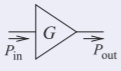
Figure \(\PageIndex{1}\)

1. What is the input power in \(\text{dBm}\)?
   \[\label{eq:3}P_{\text{in}}=2\text{ mW} = 10\cdot\log\left(\frac{2\text{ mW}}{1\text{ mW}}\right) = 10\cdot\log (2) = 3.010\text{ dBm}\approx 3.0\text{ dBm} \]
2. What is the gain, \(G\), of the amplifier in \(\text{dB}\)?
   The amplifier gain (by default this is power gain) is
   \[\label{eq:4}G=20=10\cdot\log (20)\text{ dB}=10\cdot 1.301\text{ dB}=13.0\text{ dB} \]
3. What is the output power of the amplifier?
   \[\label{eq:5}G=\frac{P_{\text{out}}}{P_{\text{in}}},\quad\text{and in decibels }G|_{\text{dB}}=P_{\text{out}}|_{\text{dBm}}-P_{\text{in}}|_{\text{dBm}} \]
   Thus the output power in \(\text{dBm}\) is
   \[\label{eq:6}P_{\text{out}}|_{\text{dBm}}=G|_{\text{dB}}+P_{\text{in}}|_{\text{dBm}}=13.0\text{ dB} +3.0\text{ dBm} =16.0\text{ dBm} \]
   Note that \(\text{dB}\) and \(\text{dBm}\) are dimensionless but they do have meaning; \(\text{dB}\) indicates a power ratio but \(\text{dBm}\) refers to a power. Quantities in \(\text{dB}\) and one quantity in \(\text{dBm}\) can be added or subtracted to yield \(\text{dBm}\), and the difference of two quantities in \(\text{dBm}\) yields a power ratio in \(\text{dB}\).

In Examples \(\PageIndex{2}\) and \(\PageIndex{3}\) two digits following the decimal point were used for the output power expressed in \(\text{dBm}\). This corresponds to an implied accuracy of about \(0.01\%\) or \(4\) significant digits of the absolute number. This level of precision is typical for the result of an engineering calculation.

Example \(\PageIndex{4}\): Power Calculations

The output stage of an RF front end consists of an amplifier followed by a filter and then an antenna. The amplifier has a gain of \(33\text{ dB}\), the filter has a loss of \(2.2\text{ dB}\), and of the power input to the antenna, \(45\%\) is lost as heat due to resistive losses. If the power input to the amplifier is \(1\text{ W}\), then:

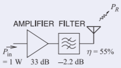
Figure \(\PageIndex{2}\)

1. What is the power input to the amplifier expressed in \(\text{dBm}\)?
   \(P_{\text{in}}=1\text{ W}=1000\text{ mW},\quad P_{\text{dBm}}=10\log (1000/1)=30\text{ dBm}\)
2. Express the loss of the antenna in \(\text{dB}\).
   \(45\%\) of the power input to the antenna is dissipated as heat.
   The antenna has an efficiency, \(\eta\), of \(55\%\) and so \(P_{2} = 0.55P_{1}\).
   \(\text{Loss} = P_{1}/P_{2} = 1/0.55 = 1.818 = 2.60\text{ dB}\).
3. What is the total gain of the RF front end (amplifier + filter + antenna)?
   \[\label{eq:7}\text{Total gain }= (\text{amplifier gain})_{\text{dB}}+(\text{filter gain})_{\text{dB}}-(\text{loss of antenna})_{\text{dB}}=(33-2.2-2.6)\text{ dB}=28.2\text{ dB} \]
4. What is the total power radiated by the antenna in \(\text{dBm}\)?
   \[\label{eq:8}P_{r}=P_{\text{in|dBm}}+(\text{amplifier gain})_{\text{dB}}+(\text{filter gain})_{\text{dB}}-(\text{loss of antenna})_{\text{dB}}=30\text{ dBm}+(33-2.2-2.6)\text{ dB}=58.2\text{ dBm} \]
5. What is the total power radiated by the antenna?
   \[\label{eq:9}P_{R}=10^{58.2/10}=(661\times 10^{3})\text{ mW}=661\text{ W} \]