2.6: The RF Link

The RF link is between a transmit antenna and a receive antenna. Sometimes the RF link includes the antenna, this will be clear from the context, but usually it includes the antennas. The principle source of link loss is the spreading out of the EM field as it propagates. In the absence obstructions the power density reduces as \(1/d^{2}\), where \(d\) is distance, and this is the line-of-sight (LOS) situation. In this section the propagation path is first described along with its impairments including propagation on multiple paths between a transmit antenna and a receive antenna.

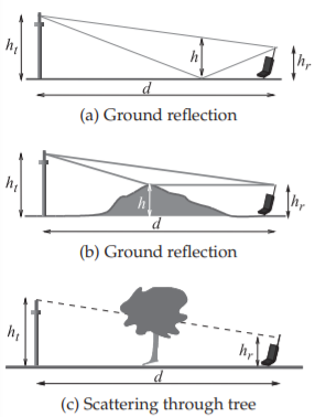
Figure \(\PageIndex{1}\): Common paths contributing to multipath propagation.

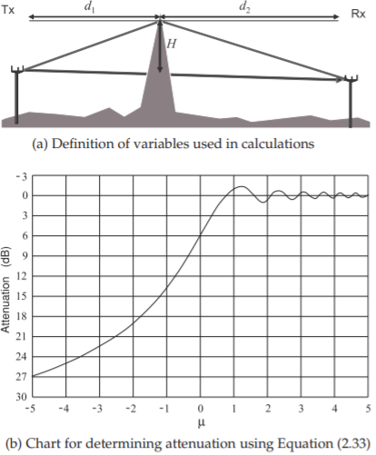
Figure \(\PageIndex{2}\): Knife-edge diffraction.

2.6.1 Propagation Path

When the radiated signal reflects and diffracts there are multiple propagation paths that result in fading as the paths constructively and destructively combine at the receiver. Of these destructive combining is much worse as it can reduce a signal level below what it would be if propagation was in free space. In urban areas, \(10\) or \(20\) paths can have significant powers [4].

Common paths encountered in cellular radio are shown in Figure \(\PageIndex{1}\). As a rough guide, in the single-digit gigahertz range each diffraction and scattering event reduces the signal received by \(20\text{ dB}\). The knife-edge diffraction scenario is shown in more detail in Figure \(\PageIndex{2}\). This case is fairly easy to analyze and can be used to estimate the effects of individual obstructions. The diffraction model is derived from the theory of half-infinite screen diffraction [5]. First, calculate the parameter \(\nu\) from the geometry of the path using

\[\label{eq:2.6.1}\nu =-H\sqrt{\frac{2}{\lambda}\left(\frac{1}{d_{1}}+\frac{1}{d_{2}}\right)} \]

Next, consult the plot in Figure \(\PageIndex{2}\)(b) to obtain the diffraction loss (or attenuation). This loss should be added (using decibels) to the otherwise determined path loss to obtain the total path loss.

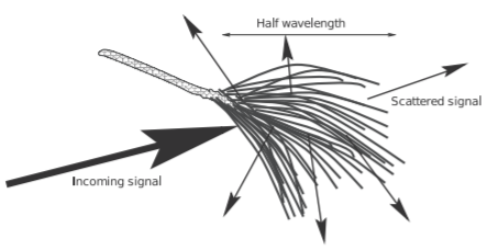
Figure \(\PageIndex{3}\): Pine needles scattering an incoming EM signal.

2.6.2 Resonant Scattering

Propagation is rarely from point to point, i.e. non-LOS (NLOS), as the path is often obstructed. One type of event that reduces transmission is scattering. The level of the effect depends on the size of the objects causing scattering. Here the effect of the pine needles of Figure \(\PageIndex{3}\) will be considered. The pine needles (as most objects in the environment) conduct electricity, especially when wet. When an EM field is incident an individual needle acts as a wire antenna, with the current maximum when the pine needle is one-half wavelength long. At this length, the “needle” antenna supports a standing wave and will re-radiate the signal in all directions. This is scattering, and there is a considerable loss in the direction of propagation of the original fields. The effect of scattering is frequency and size dependent. A typical pine needle is \(15\text{ cm}\) long, which is exactly \(\lambda /2\) at \(1\text{ GHz}\), and so a stand of pine trees have an extraordinary impact on cellular communications at \(1\text{ GHz}\). As a rough guide, \(20\text{ dB}\) of a signal is lost when passing through a small stand of pine trees.

2.6.3 Fading

Fading refers to the variation of the received signal with time or when the position of transmit or receive antennas is changed. The most important fading types are flat fading, multipath fading, and rain fading.

Flat Fading

Temperature variations of the atmosphere between the transmit and receive antennas give rise to what is called flat fading and sometimes called thermal fading. This fading is called flat because it is independent of frequency. One form of flat fading is due to refraction, which occurs when different layers of the atmosphere have different densities and thus dielectric permittivities increasing or decreasing away from the surface of the earth. The temperature profile can increase away from the earth surface or reduce depending on whether the temperature of the earth is higher than that of the air and is commonly associated with the beginning and end of the day. This causes refraction of the propagating wave, , see Figure \(\PageIndex{4}\)(a). Temperature inversions can also occur where the temperature profile producing a layer with a relatively higher permittivity. RF energy gets trapped in this layer, reflecting from the top and bottom of the inversion layer, see Figure \(\PageIndex{4}\)(b). This is called ducting. In point-to-point communication systems the transmit and receive antennas are mounted high on towers and then

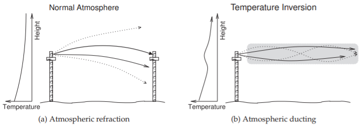
Figure \(\PageIndex{4}\): Fading resulting from ducting: (a) normal atmospheric refraction (normally the temperature of air drops with increasing height and the lower refractive index at high heights results in a concave refraction); and (b) atmospheric ducting (resulting from temperature inversion inducing an air layer with higher dielectric constant than the surrounding air).

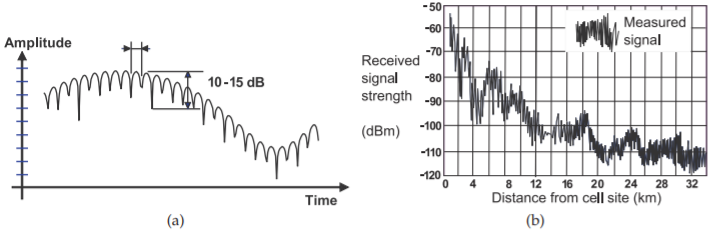
Figure \(\PageIndex{5}\): Fast and slow fading: (a) in time as a radio and obstructions move; and (b) in distance.

reflection from ground objects is often small. In such cases flat fading is the most commonly observed phenomena and minor fluctuations of several decibels in receive signal level are common throughout the day. However, when temperature variations are extreme, ducting can severely impact communications reducing signal levels by up to \(20\text{ dB}\).

Shadow Fading

Shadow fading occurs when the LOS path is blocked by an obstruction such as a building or hill. This results in relatively slow fades with the amplitude response varying in time and distance as shown in Figure \(\PageIndex{5}\). This figure shows both fast fades that are \(10\) to \(15\text{ dB}\) deep and slow or shadow fades that are \(20\) to \(30\text{ dB}\) deep.

Multipath Fading

Multipath describes the situation situations where there are many reflections that combine destructively and constructively. Multipath fading is also called fast fading, as the characteristics of the channel can change significantly in a few milliseconds. Multipath fading of \(20\text{ dB}\) can occur for a small percentage of the time on time scales of many seconds when there are few propagation paths (e.g. in a rural area) to a large percentage of the time many times per second in a dense urban environment where there are many paths. Constructive combining does increase the signal level momentarily, but there is no advantage to this. Destructive combining can result in deep fades of \(20\text{ dB}\) impacting communications and forcing the communication system to accommodate either by using higher average powers or using strategies such as multiple antennas or spreading the communication signal over a wide bandwidth since fades tend to be \(500\text{ kHz}\) to \(1\text{ MHz}\) wide at all frequencies.

When the signal on one of the paths dominates, this is usually the LOS path, fading is called Rician fading. With LOS and a single ground reflection, the situation is the classic Rician fading shown in Figure \(\PageIndex{6}\)(a). Here the ground changes the phase of the signal upon reflection by \(180^{\circ}\). When the receiver is a long way from the base station, the lengths of the two paths are almost identical and the level of the signals in the two paths are almost the same. The net result is that these two signals almost cancel, and so instead of the power falling off by \(1/d^{2}\), it falls off by \(1/d^{3}\). When there are many paths and all have similar amplitude signals, fading is called Rayleigh fading. In an urban area such as that shown in Figure \(\PageIndex{6}\)(b), there are many significant multipaths and the power falls off by \(1/d^{4}\) and sometimes faster.

Rain Fading

Rain fading is due to both the amount of rain and the size of individual rain drops and fading occurs over periods of minutes to hours. Propagation through the atmosphere is affected by absorption by molecules in the air, fog, and rain, and by scattering by rain drops. Figure 1.1.2 shows the attenuation in decibels per kilometer from \(3\text{ GHz}\) to \(300\text{ GHz}\). The attenuation due to rain increases with frequency and this derives largely from scattering.

Summary of Fading

The fades of most concern in a mobile wireless system are the deep fades resulting from destructive interference of multiple reflections. These fades vary rapidly (over a few milliseconds) if a handset is moving at vehicular speeds but occur slowly when the transmitter and receiver are fixed. Fades can be viewed as deep amplitude modulation, and so so modulation is restricted to phase shift keying schemes when a transmitter and receive

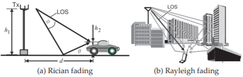
Figure \(\PageIndex{6}\): Multipath propagation: (a) line of sight (LOS) and ground reflection paths only; and (b) in an urban environment.

moving at vehicular speeds relative to each other.

2.6.4 Link Loss and Path Loss

With transmit and receive antennas included in the RF link, the usual case, link loss is defined as the ratio of the power input to the transmit antenna, \(P_{T}\), to the power delivered by the receive antenna, \(P_{R}\). Rearranging Equation (2.5.17) the total line-of-sight (LOS) link loss, \(L_{\text{LINK,LOS}}\), between the input of the transmit antenna and the output of the receive antenna separated by distance \(d\) is (in decibels):

\[\begin{align} \label{eq:2} L_{\text{LINK,LOS}}|_{\text{dB}}&=10\log\left(\frac{P_{T}}{P_{R}}\right)=10\log\left(\frac{P_{T}}{P_{D}A_{R}}\right) \\ \label{eq:3} &=10\log\left[P_{T}\left(\frac{4\pi d^{2}}{P_{T}G_{T}}\right)\left(\frac{4\pi}{\lambda ^{2}G_{R}}\right) \right] \\ \label{eq:4} &=10\log\left[\left(\frac{1}{G_{T}G_{R}}\right)\left(\frac{4\pi d}{\lambda}\right)^{2}\right] \\ \label{eq:5} &=-10\log G_{T}-10\log G_{R}+20\log\left(\frac{4\pi d}{\lambda }\right) \end{align} \]

The last term includes \(d\) and is called the LOS path loss (in decibels):

\[\label{eq:6} L_{\text{PATH,LOS}}|_{\text{dB}}=20\log\left(\frac{4\pi d}{\lambda}\right) \]

This is the preferred form of the expression for path loss, as it can be used directly in calculating link loss using the antenna gains of the transmit and receive antennas without the exercise of calculating the effective aperture size of the receive antenna.

Multipath effects result in losses that are proportional to \(d^{n}\) [6, 7] so that the general path loss, including multipath effects, is (in decibels)

\[\begin{align} L_{\text{PATH}}|_{\text{dB}}&=L_{\text{PATH,LOS}}|_{\text{dB}}+\text{excess loss}|_{\text{dB}} \nonumber \\&=20\log\left(\frac{4\pi d}{\lambda}\right) + 10(n-2)\log\left(\frac{d}{1\text{ m}}\right) \nonumber \\ &=20\log\left[\frac{4\pi(1\text{ m})}{\lambda}\right]+10(2)\log\left(\frac{d}{1\text{ m}}\right)+10(n-2)\log\left(\frac{d}{1\text{ m}}\right)\nonumber \\ \label{eq:7}&=10n\log\left[ d/(1\text{ m})\right]+C\end{align} \]

where the distance \(d\) and wavelength \(\lambda\) are in meters, and \(C\) is a constant that captures the effect of wavelength. Here,

\[\label{eq:8}C=20\log\left[ 4\pi (1\text{ m})/\lambda\right] \]

Combining this with Equation \(\eqref{eq:5}\) yields the link loss:

\[\label{eq:9}L_{\text{LINK}}|_{\text{dB}}=-G_{T}|_{\text{dB}}-G_{R}|_{\text{dB}}+10n\log [d/(1\text{ m})]+C \]

Example \(\PageIndex{1}\): Link Loss

A \(5.6\text{ GHz}\) communication system uses a transmit antenna with an antenna gain \(G_{T}\) of \(35\text{ dB}\) and a receive antenna with an antenna gain \(G_{R}\) of \(6\text{ dB}\). If the distance between the antennas is \(200\text{ m}\), what is the link loss if the power density reduces as \(1/d^{3}\)? The link loss here is between the input to the transmit antenna and the output from the receive antenna.

Solution

The link loss is provided by Equation \(\eqref{eq:9}\),

\[L_{\text{LINK}}|_{\text{dB}}=-G_{T}-G_{R}+10n\log [d/(1\text{ m})]+C\nonumber \]

and \(C\) comes from Equation \(\eqref{eq:8}\), where \(\lambda =5.36\text{ cm}\). So

\[C=20\log\left(\frac{4\pi}{\lambda}\right)=20\log\left(\frac{4\pi}{0.0536}\right)=47.4\text{ dB}\nonumber \]

With \(n=3\) and \(d=200\text{ m}\),

\[L_{\text{LINK}}|_{\text{dB}}=-35-6+10\cdot 3\cdot\log (200)+47.4\text{ dB}=75.4\text{ dB}\nonumber \]

Example \(\PageIndex{2}\): Radiated Power Density

In free space, radiated power density drops off with distance \(d\) as \(1/d^{2}\). However, in a terrestrial environment there are multiple paths between a transmitter and a receiver, with the dominant paths being the direct LOS path and the path involving reflection off the ground. Reflection from the ground partially cancels the signal in the direct path, and in a semi-urban environment results in an attenuation loss of \(40\text{ dB}\) per decade of distance (instead of the \(20\text{ dB}\) per decade of distance roll-off in free space). Consider a transmitter that has a power density of \(1\text{ W/m}^{2}\) at a distance of \(1\text{ m}\) from the transmitter.

1. The power density falls off as \(1/d^{n}\), where \(d\) is distance and \(n\) is an index. What is \(n\)?
2. At what distance from the transmit antenna will the power density reach \(1\:\mu\text{W}\cdot\text{m}^{-2}\)?

Solution

1. Power drops off by \(40\text{ dB}\) per decade of distance. \(40\text{ dB}\) corresponds to a factor of \(10,000 (= 10^{4})\). So, at distance \(d\), the power density \(P_{D}(d) = k/d^{n}\) (\(k\) is a constant). At a decade of distance, \(10d\), \(P_{D}(10d) = k/(10d)^{n} = P_{D}(d)/10000\), thus
   \[\frac{k}{10^{n}d^{n}}=\frac{1}{10,000}\frac{k}{d^{n}};\quad 10^{n}=10,000\Rightarrow n=4\nonumber \]
2. At \(d=1\text{ m}\), \(P_{D}(1\text{ m})=1\text{ W/m}^{2}\). At a distance \(x\),
   \[P_{D}(x)=1\:\mu\text{W/m}^{2}=\frac{k}{x^{4}}\text{m}^{2}=\frac{k}{x^{4}}\to x^{4}=\frac{1}{10^{-6}}\quad\text{and so}\quad x=31.6\text{ m}\nonumber \]

2.6.5 Propagation Model in the Mobile Environment

RF propagation in the mobile environment cannot be accurately derived. Instead, a fit to measurements is often used. One of the models is the Okumura–Hata model [8], which calculates the path loss as

\[\label{eq:10} L_{\text{PATH}}|_{\text{(dB)}}=69.55+26.16\log f-13.82\log H+(44.9-6.55\log H)\cdot\log d+c \]

where \(f\) is the frequency (in \(\text{MHz}\)), \(d\) is the distance between the base station and terminal (in \(\text{km}\)), \(H\) is the effective height of the base station antenna (in \(\text{m}\)), and \(c\) is an environment correction factor (\(c = 0\text{ dB}\) in a dense urban area, \(c = −5\text{ dB}\) in an urban area, \(c = −10\text{ dB}\) in a suburban area, and \(c = −17\text{ dB}\) in a rural area, for \(f = 1\text{ GHz}\) and \(H=1.5\text{ m}\)).

There are many propagation models for different frequency ranges and different environments. The considerable effort put into developing reliable models is because being able to predict signal coverage is essential to efficient design of basestation layout.