3.1: Introduction

A transmission line stores electric and magnetic energy. As such a line has a circuit form that combines inductors, \(L_{s}\) (for the magnetic energy), capacitors, \(C_{s}\) (for the electric energy), and resistors, \(R_{s}\) (modeling losses), whose values depend on the line geometry and material properties.

The transmission lines considered in this chapter are restricted to just two parallel conductors, as shown in Figure \(\PageIndex{1}\), with the distance between the two wires (i.e., in the transverse direction) being substantially smaller than the wavelengths of the signals on the line. The correct physical interpretation is that the conductors of a transmission line confine and guide an EM field. The EM field contains the energy of the signal and not the current on the line. However, with electrically small transverse dimensions, a two conductor line

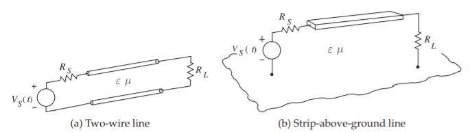
Figure \(\PageIndex{1}\): Two conductor transmission lines.

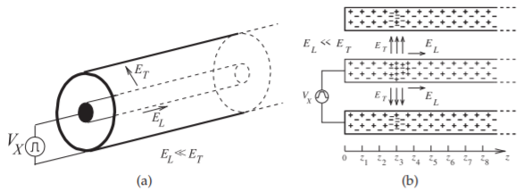
Figure \(\PageIndex{2}\): A coaxial transmission line: (a) three-dimensional view; (b) the line with pulsed voltage source showing the electric fields at an instant in time as a voltage pulse travels down the line.

may be satisfactorily analyzed on the basis of voltages and currents.

Frequency-domain analysis is the best way to understand transmission lines. This transmission line theory with modern developments is presented in Section 3.2 and useful formulas and concepts are developed in Section 3.3 for lossless transmission lines. Section 3.4 presents several configurations of lossless lines that are particularly useful in microwave circuit design and used in many places in this book series.

3.1.1 When Must a Line be Considered a Transmission Line

The key determinant of whether a transmission line can be considered as an invisible connection between two points is whether the signal anywhere along the interconnect has the same value at a particular instant. If the value of the signal (say, voltage) varies along the line (at an instant), then it may be necessary to consider transmission line effects. A typical criterion used is that if the length of the interconnect is less than \(1/20\text{th}\) of the wavelength of the highest-frequency component of a signal, then transmission line effects can be safely ignored and the circuit can be modeled as a single \(RLC\) circuit [1].

3.1.2 Movement of a Signal on a Transmission Line

When a positive voltage pulse is applied to the center conductor of a coaxial line, as shown in Figure \(\PageIndex{2}\)(a), an electric field results that is directed from the center conductor to the outer conductor. Referring to Figure \(\PageIndex{2}\)(b), the component of the field that is directed along the shortest path from the center conductor to the outer conductor is denoted \(E_{T}\), and the subscript \(T\) denotes the transverse component of the field as shown. Figure \(\PageIndex{2}\)(b) shows the fields in the structure after the pulse has started moving along the line. This is shown in another view in Figure \(\PageIndex{3}\) at four different times. The transverse voltage, \(V_{T}\), is given by \(E_{T}\) integrated along a path between the inner and outer conductors: \(V_{T} ≈ E_{T} (a − b)\). This is a good measure, provided that the transverse dimensions are small compared to a wavelength. The voltage pulse exciting the line has a trapezoidal shape and the voltage between the inner and outer conductor has the same form as \(E_{T}\). As indicated by Maxwell’s equations, a change in time of the electric field results in a spatial

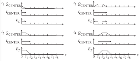
Figure \(\PageIndex{3}\): Fields, currents, and charges on the coaxial transmission line of Figure \(\PageIndex{2}\) at times \(t_{4} > t_{3} > t_{2} > t_{1}\). \(Q_{\text{CENTER}}\) is the net free charge on the center conductor. \(I_{\text{CENTER}}\) is the current on the center conductor.

change in the magnetic field and hence current. As a result there is a variation of the current in time and this results in a spatial change of the electric field. The chasing from a time variation to a spatial variation and then back to a time variation causes the pulse to move down the line.

The pulse moves down the line at the group velocity, which for a lossless coaxial line is the same as the phase velocity, \(v_{p}\)\(^{1}\). This is determined by the physical properties of the region between the conductors. The permittivity, \(\varepsilon\), describes energy storage associated with the electric field, \(E\), and the energy storage associated with the magnetic field, \(H\), is described by the permeability, \(\mu\). It has been determined that

\[\label{eq:1}v_{p}=1/\sqrt{\mu\varepsilon} \]

In free space \(v_{p} = c = 1/\sqrt{\mu_{0}\varepsilon_{0}} = 3\times 10^{8}\text{ m/s}\). The free-space wavelengths, \(\lambda_{0} = c/f\), at several frequencies, \(f\), are

\(f\)	\(100\text{ MHz}\)	\(1\text{ GHz}\)	\(10\text{ GHz}\)
\(\lambda_{0}\)	\(3\text{ m}\)	\(30\text{ cm}\)	\(3.0\text{ cm}\)

Table \(\PageIndex{1}\)

Example \(\PageIndex{1}\): Transmission Line Wavelength

A length of coaxial line is filled with a dielectric having a relative permittivity, \(\varepsilon_{r}\), of \(20\) and is designed to be \(1/4\) wavelength long at a frequency, \(f\), of \(1.850\text{ GHz}\). \((\mu_{r} = 1)\)

1. What is the free-space wavelength?
2. What is the wavelength of the signal in the dielectric-filled coaxial line?
3. How long is the line?

Solution

1. \(\lambda_{0}=c/f=3\times 10^{8}/1.85\times 10^{9}=0.162\text{ m}=16.2\text{ cm}\)
2. Note that for a dielectric-filled line with \(\mu_{r}=1,\:\lambda =v_{p}/f=c/(\sqrt{\varepsilon_{r}}f)=\lambda_{0}/\sqrt{\varepsilon_{r}}\), so \(\lambda =\lambda_{0}/\sqrt{\varepsilon_{r}}=16.2\text{ cm}/\sqrt{20}=3.62\text{ cm}\)
3. \(\lambda_{g}/4=3.62\text{ cm}/4=9.05\text{ mm}\)

Footnotes

[1] The phase velocity is the apparent velocity of a point of constant phase on a sinewave and is almost frequency independent for a low-loss coaxial line of small transverse dimensions (less than \(\lambda /10\)).