3.3: The Lossless Terminated Line

Microwave engineers want to work with total voltage and current when possible and the art of design synthesis usually requires relating the total voltage and current world of a lumped element circuit to the traveling voltage world of transmission lines. This section develops the important abstractions that enable the total voltage and current view of the world to be used with transmission lines. The first step is in Section 3.3.1 where total voltages and currents are related to forward- and backward-traveling voltages and currents. Insight into traveling waves and reflections is presented in Section 3.3.2. Important abstractions are presented first for the input reflection coefficient of a terminated lossless line in Section 3.3.3 and then for the input impedance of the line in Section 3.3.4. The last section, Section 3.3.5, presents a view of the total voltage on the transmission line and describes the voltage standing wave concept.

Total Voltage and Current on the Line

Consider the terminated line shown in Figure \(\PageIndex{1}\)(a). Assume an incident or forward-traveling wave, with traveling voltage \(V_{0}^{+}e^{-\jmath\beta z}\) and current \(I_{0}^{+}e^{-\jmath\beta z}\) propagating toward the load \(Z_{L}\) at \(z = 0\). The characteristic impedance of the transmission line is the ratio of the voltage and current traveling waves so that

\[\label{eq:1} \frac{V_{0}^{+}(z)}{I_{0}^{+}(z)}=\frac{V_{0}^{+}e^{-\jmath\beta z}}{I_{0}^{+}e^{-\jmath\beta z}}=\frac{V_{0}^{+}(0)}{I_{0}^{+}(0)}=\frac{V_{0}^{+}}{I_{0}^{+}}=Z_{0} \]

The reflected wave has a similar relationship (but note the sign change):

\[\label{eq:2}\frac{V_{0}^{-}e^{\jmath\beta z}}{-I_{0}^{-}e^{\jmath\beta z}}=\frac{V_{0}^{-}}{-I_{0}^{-}}=Z_{0} \]

The load \(Z_{L}\) imposes an additional constraint on the relationship of the total voltage and current at \(z = 0\):

\[\label{eq:3}\frac{V_{L}}{I_{L}}=\frac{V(z=0)}{I(z=0)}=Z_{L} \]

When \(Z_{L}\neq Z_{0}\) there must be a reflected wave with appropriate amplitude to satisfy the above equations. Now the total voltage

\[\label{eq:4}V(z)=V_{0}^{+}e^{-\jmath\beta z}+V_{0}^{-}e^{\jmath\beta z} \]

and the total current, \(I(z)\), is related to the traveling current waves by

\[\label{eq:5}I(z)=\frac{V_{0}^{+}}{Z_{0}}e^{-\jmath\beta z}-\frac{V_{0}^{-}}{Z_{0}}e^{\jmath\beta z}=I_{0}^{+}e^{-\jmath\beta z}+I_{0}^{-}e^{\jmath\beta z} \]

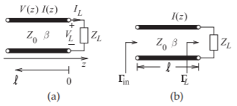
Figure \(\PageIndex{1}\): A terminated transmission line.

Thus at the termination of the line (\(z = 0\)),

\[\frac{V(0)}{I(0)}=Z_{L}=Z_{0}\frac{V_{0}^{+}+V_{0}^{-}}{V_{0}^{+}-V_{0}^{-}}\nonumber \]

This can be rearranged as the ratio of the reflected voltage to the incident voltage:

\[\frac{V_{0}^{-}}{V_{0}^{+}}=\frac{Z_{L}-Z_{0}}{Z_{L}+Z_{0}}\nonumber \]

This ratio is defined as the voltage reflection coefficient at the load,

\[\label{eq:6}\Gamma_{L}=\Gamma_{L}^{V}=\frac{V_{0}^{-}(0)}{V_{0}^{+}(0)}=\frac{V_{0}^{-}}{V_{0}^{+}}=\frac{Z_{L}-Z_{0}}{Z_{L}+Z_{0}} \]

That is, at the load

\[\label{eq:7}V_{0}^{-}=\Gamma_{L}V_{0}^{+} \]

The relationship in Equation \(\eqref{eq:6}\) can be rewritten so that the input load impedance can be obtained from the reflection coefficient:

\[\label{eq:8}Z_{L}=Z_{0}\frac{1|\Gamma^{V}}{1-\Gamma^{V}} \]

Similarly, the current reflection coefficient can be written as

\[\label{eq:9}\Gamma^{I}=\frac{I_{0}^{-}}{I_{0}^{+}}=\frac{-Z_{L}+Z_{0}}{Z_{L}+Z_{0}}=-\Gamma^{V} \]

The voltage reflection coefficient is used most of the time, so the reflection coefficient, \(\Gamma\), on its own refers to the voltage reflection coefficient, \(\Gamma^{V}=\Gamma\).

Example \(\PageIndex{1}\): Forward- and Backward-Traveling Waves at an Open Circuit

A lossless transmission line is terminated in an open circuit. What is the relationship between the forward- and backward-traveling voltage waves at the end of the line?

Solution

At the end of the line the total current is zero, so that \(I^{+} + I^{−} = 0\) and so

\[\label{eq:10}I^{-}=-I^{+} \]

The forward- and backward traveling voltages and currents are related to the characteristic impedance by

\[\label{eq:11}Z_{0}=V^{+}/I^{+}=-V^{-}/I^{-} \]

Note the change in sign, as a result of the direction of propagation changing but the positive reference for current is in the same direction. Substituting for \(I^{-}\) at the termination,

\[\label{eq:12}V^{+}=-V^{-}I^{+}/I^{-}=-V^{-}I^{+}/(-I^{+})=V^{-} \]

Thus the total voltage at the end of the line, \(V_{TOTAL}\), is \(V^{+} + V^{-} = 2V^{+}\). Note that the total voltage at the end of the line is twice the incident (forward-traveling) voltage.

Example \(\PageIndex{2}\): Current Reflection Coefficient

A load consists of a shunt connection of a capacitor of \(10\text{ pF}\) and a resistor of \(60\:\Omega\). The load terminates a lossless \(50\:\Omega\) transmission line. The operating frequency is \(5\text{ GHz}\).

1. What is the impedance of the load?
2. What is the normalized impedance of the load (normalized to \(Z_{0}\) of the line)?
3. What is the reflection coefficient of the load?
4. What is the current reflection coefficient of the load?

Solution

1. \(C=10\cdot 10^{-12}\text{ F},\: R=60\:\Omega ;\:f=5\cdot 10^{9}\text{ Hz};\:\omega =2\pi f;\: Z_{0}=50\:\Omega\)
   \[Z_{L}=R||C=(1/R +\jmath\omega C)^{-1}=0.168-\jmath 3.174\:\Omega\nonumber \]
2. \(z_{L}=Z_{L}/Z_{0}=3.368\cdot 10^{-3}-\jmath 0.063\)
3. This is the voltage reflection coefficient. \(\Gamma_{L}=(z_{L}-1)/(z_{L}+1)=-0.985-\jmath 0.126 =0.993\angle 187.3^{\circ}\).
4. \(\Gamma_{L}^{I}=-\Gamma_{L}= 0.985 + \jmath 0.126 = 0.993\angle (187.3 − 180)^{\circ} = 0.993\angle 7.3^{\circ}\).

3.3.2 Forward- and Backward-Traveling Pulses

Reflections at the end of a line produce a backward-traveling signal. Forward- and backward-traveling pulses are shown in Figure \(\PageIndex{2}\)(a) for the situation where the resistance at the end of the line is lower than the

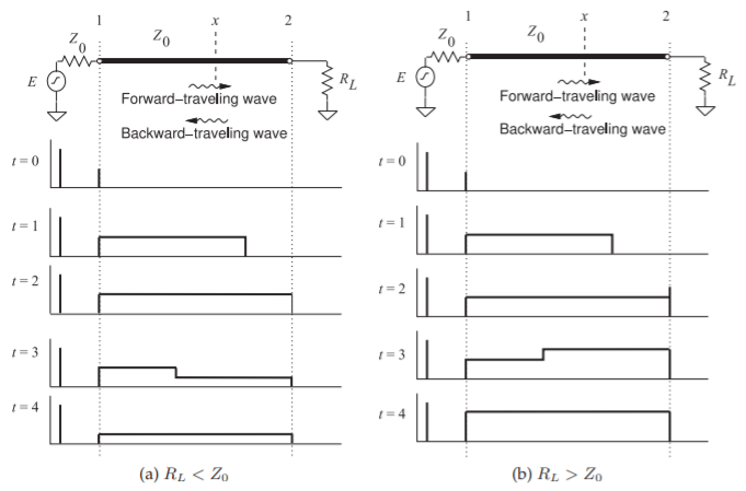
Figure \(\PageIndex{2}\): Reflection of a voltage pulse from a load: (a) when the resistance of the load, \(R_{L}\) is lower than the characteristic impedance of the line, \(Z_{0}\); and (b) when \(R_{L}\) is greater than \(Z_{0}\).

characteristic impedance of the line (\(Z_{L} < Z_{0}\)). The voltage source is a step voltage that is zero for time \(t < 0\). At time \(t = 0\), the step is applied to the line and it begins traveling down the line, as shown at time \(t = 1\). This voltage step moving from left to right is called the forward-traveling voltage wave.

At time \(t = 2\), the leading edge of the step reaches the load, and as the load has lower resistance than the characteristic impedance of the line, the total voltage across the load drops below the level of the forward-traveling voltage step. The reflected wave is called the backward-traveling wave and it must be negative, as it adds to the forward-traveling wave to yield the total voltage. Thus the voltage reflection coefficient, \(\Gamma\), is negative and the total voltage on the line, which is all that can be directly observed, drops. A reflected, smaller, and opposite step signal travels in the backward direction and adds to the forward-traveling step to produce the waveform shown at \(t = 3\). The impedance of the source matches the transmission line impedance so that the reflection at the source is zero. The signal on the line at time \(t = 4\), the time for round-trip propagation on the line, therefore remains at the lower value. The easiest way to remember the polarity of the reflected pulse is to consider the situation with a short-circuit at the load. Then the total voltage on the line at the load must be zero. The only way this can occur when a signal is incident is if the reflected signal is equal in magnitude but opposite in sign, in this case \(\Gamma = −1\). So whenever \(|Z_{L}| < |Z_{0}|\), the reflected pulse will tend to subtract from the incident pulse.

The opposite situation occurs when the resistance at the load is higher than the characteristic impedance of the line (Figure 3-9(b)). In this case the reflected pulse has the same polarity as the incident signal. Again, to remember this, think of the open-circuited case. The voltage across the load doubles, as the reflected pulse has the same sign as well as magnitude as that of the incident signal, in this case \(\Gamma = +1\). This is required so that the total current is zero.

A more illustrative situation is shown in Figure \(\PageIndex{3}\), where a more complicated signal is incident on a load that has a resistance higher than that of the characteristic impedance of the line. The peaking of the voltage that results at the load is typically the design objective in many long digital interconnects, as less overall signal energy needs to be transmitted down the line, or equivalently a lower current drive capability of the source is required to achieve first incidence switching. This is at the price of having reflected signals on the interconnects, but these are dissipated through a combination of line loss and absorption of the reflected signal at the driver.

3.3.3 Input Reflection Coefficient of a Lossless Line

The reflection coefficient looking into a line varies with position along the line as the forward- and backward-traveling waves change in relative phase. Referring to Figure \(\PageIndex{4}\), at a distance ℓ from the load (i.e., \(z = −\ell\)), the input reflection looking into a terminated lossless line is

\[\label{eq:13} \Gamma_{\text{in}}|_{z=-\ell}=\frac{V^{-}(z=-\ell)}{V^{+}(z=-\ell)}=\frac{V^{-}(z=0)e^{-\jmath\beta\ell}}{V^{+}(z=0)e^{+\jmath\beta\ell}}=\frac{V^{-}(z=0)e^{-\jmath\beta\ell}}{V^{+}(z=0)e^{+\jmath\beta\ell}}=\Gamma_{L}e^{-\jmath\beta\ell} \]

Note that \(\Gamma_{\text{in}}\) has the same magnitude as \(\Gamma_{L}\) but rotates in the clockwise direction (becomes increasingly negative) at twice the rate of increase of the

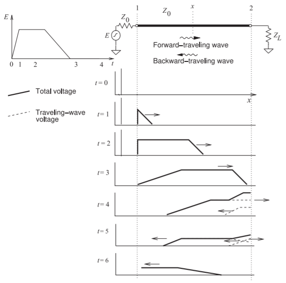
Figure \(\PageIndex{3}\): Reflection of a pulse from a termination with \(Z_{L} > Z_{0}\). \(Z_{L}\) and \(Z_{0}\) are real.

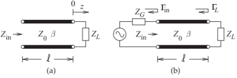
Figure \(\PageIndex{4}\): Terminated transmission line: (a) a transmission line terminated in a load impedance, \(Z_{L}\), with an input impedance of \(Z_{\text{in}}\); and (b) a transmission line with source impedance \(Z_{G}\) and load \(Z_{L}\).

electrical length \(\beta\ell\).

It is important to graphical concepts introduced later that there be a full appreciation for the angle of \(\Gamma_{\text{in}}\) becoming increasingly negative at twice the rate at which the electrical length of the line increases. Figure \(\PageIndex{5}\) is a way of visualizing this. The transmission line here is \(\lambda /4\) long with an electrical length of \(90^{\circ}\) and is terminated in a load with reflection coefficient \(\Gamma_{L} = +1\). At position \(z = 0\) the forward-traveling voltage wave is \(v^{+}(t, 0) = |V^{+}| \cos(\omega t)\), and this then propagates down the line in the \(+z\) direction. The forward-traveling voltage at point \(z = \lambda /8\) at \(t = 0\) will be the same as the voltage at \(z = 0\) at a time one-eighth of a period in the past. The voltage at \(z =\lambda /8\)

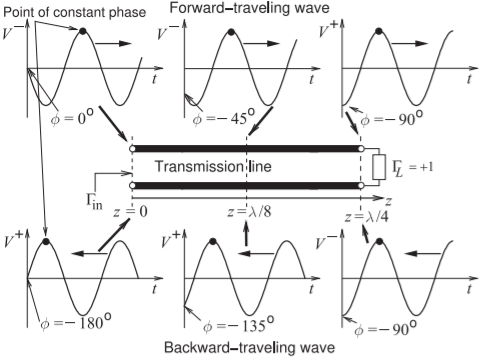
Figure \(\PageIndex{5}\): The forward-traveling wave \(v^{+}(t, z) = |V^{+}| \cos (\omega t − \beta z) = |V^{+}| \cos (\omega t + \phi (z))\) and the backward-traveling wave \(v^{−}(t, z) = |V^{+}| \cos( \omega t + \beta z) = |V^{+}| \cos [\omega t + \phi (z)]\). The phase, \(\phi\), of the forward-traveling wave becomes increasingly negative along the line as \(z\) increases, and when reflected the phase \(\phi\) of the backward-traveling wave becomes increasingly negative as the wave moves away from the load (i.e. as \(z\) decreases).

is \(v^{+}(t, \lambda /8) = |V^{+}| \cos (\omega t − 2π/8)\), i.e. there is a phase rotation of \(−45^{\circ}\). Then at \(z = \lambda /4, v^{+}(t, \lambda /4) = |V^{+}| \cos (\omega t − 2π/4)\), i.e. at time \(t = 0\) there is a phase rotation of \(−90^{\circ}\) relative to \(v^{+}(0, 0)\), and this is the negative of the electrical length of the line. The voltage wave reflects at the load and becomes a backward-traveling wave. Here \(\Gamma_{L} = +1\) and so, at the load, the phase of the backward- and forward-traveling waves are the same. The backward-traveling wave continues to travel in the \(−z\) direction and its phase at \(t = 0\) becomes increasingly negative as \(z\) gets closer to the input of the line. The phase of the backward-traveling wave at \(z = 0\) is rotated \(−90^{\circ}\) with respect to the backward-traveling wave at the load, and has rotated \(−180^{\circ}\) relative to the forward-traveling wave at \(z = 0\). For a lossless line, in general, the angle of \(\Gamma_{\text{in}} = [\text{phase of }V^{−}(z = 0)\) relative to the phase of \(V^{+}(z = 0)] + (\text{the phase of }\Gamma_{L}) = −2(\text{electrical length of the line}) + (\text{the phase of }\Gamma_{L})\).

3.3.4 Input Impedance of a Lossless Line

The impedance looking into a lossless line varies with position, as the forward- and backward-traveling waves combine to yield position-dependent total voltage and current. At a distance \(\ell\) from the load (i.e., \(z = −\ell\)), the input impedance seen looking toward the load is

\[\label{eq:14} Z_{\text{in}}|z=-\ell =\frac{V(z=-\ell)}{I(z=-\ell)}=Z_{0}\frac{I+|\Gamma |e^{\jmath (\Theta -2\beta\ell )}}{1-|\Gamma |e^{\jmath (\Theta -2\beta\ell)}}=Z_{0}\frac{1+\Gamma_{L}e^{\jmath (-2\beta\ell)}}{1-\Gamma_{L}e^{\jmath (-2\beta\ell)}} \]

Another form is obtained by substituting Equation \(\eqref{eq:6}\) in Equation \(\eqref{eq:14}\):

\[\begin{align} Z_{\text{in}}&=Z_{0}\frac{(Z_{L}+Z_{0})e^{\jmath\beta\ell}+(Z_{L}-Z_{0})e^{-\jmath\beta\ell}}{(Z_{L}+Z_{0})e^{\jmath\beta\ell}-(Z_{L}-Z_{0})e^{-\jmath\beta\ell}}=Z_{0}\frac{Z_{L}\cos (\beta\ell) +\jmath Z_{0}\cos (\beta\ell)}{Z_{0}\cos (\beta\ell )+\jmath Z_{L}\cos (\beta\ell)} \nonumber \\ \label{eq:15}&=Z_{0}\frac{Z_{L}+\jmath Z_{0}\tan\beta\ell}{Z_{0}+\jmath Z_{L}\tan\beta\ell} \end{align} \]

This is the lossless telegrapher’s equation. The electrical length, \(\beta\ell\), is in radians when used in calculations.

3.3.5 Standing Waves and Voltage Standing Wave Ratio

The total voltage on a terminated line is the sum of forward- and backwardtraveling waves. This sum produces what is called a standing wave. Figure \(\PageIndex{6}\) shows the total and traveling waveforms on a line terminated in a reactance and evaluated at times equal to multiples of an eighth of a period. Here the traveling waves have the same amplitude indicating that the termination of the line is reactive, \(|\Gamma | = 1\). The interesting property here is that the total voltage appears as a standing wave with fixed points called nodes where the total voltage is always zero. This is more easily seen in Figure \(\PageIndex{7}\)(a), where the total voltage is overlaid for many times. If the termination has resistance, then the magnitude of the backward-traveling wave will be less than that of the forward-traveling wave and the overlaid

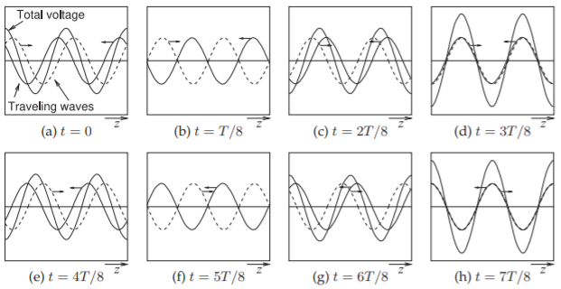
Figure \(\PageIndex{6}\): Evolution of a standing wave as the sum of forward- and backward-traveling waves (to the right and left, respectively) of equal amplitude evaluated at times \(t\) equal to eighths of the period \(T\). At \(t = T /8\) and \(t = 5T /8\) the total voltage everywhere on the line is zero.

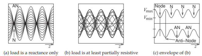
Figure \(\PageIndex{7}\): Standing waves as an overlay of waveforms at many times: (a) when the forward and backward-traveling waves have the same amplitude; (b) when the waves have different amplitudes; and (c) the envelope of the standing wave. N is a node (a minimum) and AN is an antinode (a maximum). Nodes, N, are separated by \(\lambda /2\). Antinodes, AN, are separated by \(\lambda /2\).

total voltage is as shown in Figure \(\PageIndex{7}\)(b). This is still a standing wave, but the minima are now not zero. The envelope of the standing wave is shown in Figure \(\PageIndex{7}\)(c), where there is a maximum amplitude \(V_{\text{max}}\) and a minimum amplitude \(V_{\text{min}}\).

Now this situation will be examined mathematically to relate the standing wave to the reflection coefficient. If \(\Gamma =0\), then the magnitude of the total voltage on the line, \(|V (z)|\), is equal to \(|V_{0}^{+}|\) anywhere on the line. For this reason, such a line is said to be “flat.” If there is reflection the magnitude of the total voltage on the line is not constant (see Figure \(\PageIndex{7}\)(b)). Thus from Equation \(\eqref{eq:13}\):

\[\label{eq:16}|V(z)|=|V_{0}^{+}||1+\Gamma e^{2\jmath\beta z}|=|V_{0}^{+}||1+\Gamma e^{-2\jmath\beta\ell}| \]

where \(z = −\ell\) is the positive distance measured from the load at \(z = 0\) toward the generator. Or, setting \(\Gamma = |\Gamma |e^{\jmath\Theta}\),

\[\label{eq:17}|V(z)|=|V_{0}^{+}||1+|\Gamma |e^{\jmath (\Theta -2\beta\ell)}| \]

where \(\Theta\) is the phase of the reflection coefficient (\(\Gamma = |\Gamma |e^{\jmath\Theta})\) at the load. This result shows that the voltage magnitude oscillates with position \(z\) along the line. The maximum value occurs when \(e^{\jmath (\Theta -2\beta\ell)}=1\) and is given by

\[\label{eq:18} V_{\text{max}}=|V_{0}^{+}|(1+|\Gamma |) \]

Similarly the minimum value of the total voltage magnitude occurs when the phase term is \(e^{\jmath (\Theta -2\beta\ell)}=-1\), and is given by

\[\label{eq:19} V_{\text{min}}=|V_{0}^{+}|(1-|\Gamma |) \]

A mismatch can be defined by the voltage standing wave ratio (VSWR):

\[\label{eq:20}\text{VSWR}=\frac{V_{\text{max}}}{V_{\text{min}}}=\frac{(1+|\Gamma |)}{(1-|\Gamma |)} \]

Also

\[\label{eq:21} |\Gamma |=\frac{\text{VSWR}-1}{\text{VSWR}+1} \]

Notice that in general \(\Gamma\) is complex, but \(\text{VSWR}\) is necessarily always real and \(1 ≤ \text{VSWR} ≤ ∞\). For the matched condition, \(\Gamma =0\) and \(\text{VSWR} = 1\), and the closer \(\text{VSWR}\) is to \(1\), the closer the load is to being matched to the line and the more power is delivered to the load. The magnitude of the reflection coefficient on a line with a short-circuit or open-circuit load is \(1\), and in both cases the \(\text{VSWR}\) is infinite.

To determine the position of the standing wave maximum, ℓmax, consider Equation \(\eqref{eq:17}\) and note that at the maximum

\[\label{eq:22}\Theta -2\beta\ell_{\text{max}}=2 n\pi ,\quad n=0,1,2,\ldots \]

Here \(\Theta\) is the angle of the reflection coefficient at the load:

\[\label{eq:23}\Theta -2n\pi =2\frac{2\pi}{\lambda_{g}}\ell_{\text{max}} \]

Thus the position of the voltage maxima, \(\ell_{\text{max}}\), normalized to wavelength is

\[\label{eq:24}\frac{\ell_{\text{max}}}{\lambda_{g}}=\frac{1}{2}\left(\frac{\Theta}{2\pi}-n\right),\quad n=0,-1,-2,\ldots \]

Similarly the position of the voltage minima is (using Equation \(\eqref{eq:17}\)):

\[\label{eq:25}\Theta -2\beta\ell_{\text{min}}=(2n+1)\pi \]

After rearranging the terms,

\[\label{eq:26}\frac{\ell_{\text{min}}}{\lambda_{g}}=\frac{1}{2}\left(\frac{\Theta}{2\pi}-n+\frac{1}{2}\right),\quad n=0,-1,-2,\ldots \]

Summarizing from Equations \(\eqref{eq:24}\) and \(\eqref{eq:26}\):

1. The distance between two successive maxima is \(\lambda_{g}/2\).
2. The distance between two successive minima is \(\lambda_{g}/2\).
3. The distance between a maximum and an adjacent minimum is \(\lambda_{g}/4\).
4. From the measured \(\text{VSWR}\) the magnitude of the reflection coefficient \(|\Gamma |\) can be found. From the measured \(\ell_{\text{max}}\) the angle \(\Theta\) of \(\Gamma\) can be found. Then from \(\Gamma\) the load impedance can be found.

In a similar manner to that above, the magnitude of the total current on the line is

\[\label{eq:27}|I(\ell )|=\frac{|V_{0}^{+}|}{Z_{0}}\left|1-|\Gamma |e^{\jmath (\Theta -2\beta\ell)}\right| \]

Hence the standing wave current is maximum where the standing-wave voltage amplitude is minimum, and minimum where the standing-wave voltage amplitude is maximum.

Now \(Z_{\text{in}}\) in Equation \(\eqref{eq:15}\) is a periodic function of \(\ell\) with period \(\lambda /2\) and it varies between \(Z_{\text{max}}\) and \(Z_{\text{min}}\), where

\[\label{eq:28}Z_{\text{max}}=\frac{V_{\text{max}}}{I_{\text{min}}}=Z_{0}\times\text{VSWR}\quad\text{and}\quad Z_{\text{min}}=\frac{V_{\text{min}}}{I_{\text{max}}}=\frac{Z_{0}}{\text{VSWR}} \]

Example \(\PageIndex{3}\): Standing Wave Ratio

In Example 3.3.2 a load consisted of a capacitor of \(10\text{ pF}\) in shunt with a resistor of \(60\:\Omega\). The load terminated a lossless \(50\:\Omega\) transmission line. The operating frequency is \(5\text{ GHz}\).

1. What is the SWR?
2. What is the current standing wave ratio (ISWR)? (When SWR is used on its own it is assumed to refer to VSWR.)

Solution

1. From Example 3.3.2, \(\Gamma_{L}=0.993\angle 187.3^{\circ}\) and so
   \[\text{VSWR}=\frac{1+|\Gamma_{L}|}{1-|\Gamma_{L}|}=\frac{1+0.993}{1-0.993}=285\nonumber \]
2. \(\text{ISWR}=\text{VSWR}=285\).

Example \(\PageIndex{4}\): Standing Waves

A load has an impedance \(Z_{L} = 45+\jmath 75\:\Omega\) and the system reference impedance, \(Z_{0}\), is \(100\:\Omega\).

1. What is the reflection coefficient?
2. What is the current reflection coefficient?
3. What is the SWR?
4. What is the ISWR?
5. The power available from a source with a \(100\:\Omega\) Thevenin equivalent impedance is \(1\text{ mW}\). The source is connected directly to the load, \(Z_{L}\). Use the reflection coefficient to calculate the power delivered to \(Z_{L}\).
6. What is the total power absorbed by the Thevenin equivalent source impedance?
7. Discuss the effect on power flow of inserting a lossless \(100\:\Omega\) transmission line between the source and the load.

Solution

1. The voltage reflection coefficient is
   \[\begin{align} \Gamma_{L}&=(Z_{L}-Z_{0})/(Z_{L}+Z_{0})=(45+\jmath 75-100)/(45+\jmath 75+100)\nonumber \\ &=(93.0\angle (2.204\text{ rads}))/(163.2\angle (0.4773\text{ rads}))\nonumber \\ \label{eq:29}&=0.570\angle (1.726\text{ rads}0.570\angle 98.9^{\circ}=-0.0881+\jmath 0.653=\Gamma^{V}\end{align} \]
2. The current reflection coefficient is
   \[\label{eq:30}\Gamma^{I}=-\Gamma^{V}=0.0881-\jmath 0.563=0.570\angle (98.9^{\circ}-180^{\circ})=0.570\angle 81.1^{\circ} \]
3. The SWR is the VSWR, so
   \[\label{eq:31} \text{SWR}=\text{VSWR}=\frac{V_{\text{max}}}{V_{\text{min}}}=\frac{1+|\Gamma^{V}|}{1-|\Gamma^{V}|}=\frac{1+0.570}{1-0.570}=3.65 \]
4. The current SWR is \(\text{ISWR}=\text{VSWR}\).
5. To determine the reflection coefficient of the load, begin by developing the Thevenin equivalent circuit of the load. The power available from the source is \(P_{A} = 1\text{ mW}\), so the Thevenin equivalent circuit is
   
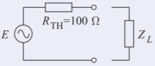
   Figure \(\PageIndex{8}\)
   The power reflected by the load is
   \[P_{R}=P_{A}|\Gamma_{L}^{2}|=1\text{ mW}\cdot (0.570)^{2}=0.325\text{ mW}\nonumber \]
   and the power delivered to the load is
   \[P_{D}=P_{A}(1-|\Gamma_{L}^{2}|)=0.675\text{ mW}\nonumber \]
6. It is tempting to think that the power dissipated in \(R_{\text{TH}}\) is just \(P_{R}\). However, this is not correct. Instead, the current in \(R_{\text{TH}}\) must be determined and then the power dissipated in \(R_{\text{TH}}\) found. Let the current through \(R_{\text{TH}cdot}\) be \(I\), and this is composed of forward and backward-traveling components:
   \[I=I^{+}+I^{-}=(1+\Gamma_{I})I^{+}\nonumber \]
   where \(I^{+}\) is the forward-traveling current wave. Thus
   \[P_{A}=\frac{1}{2}|I^{+}|^{2}R_{\text{TH}}=\frac{1}{2}|I^{+}|^{2}\times 100=1\text{ mW}=10^{-3}\text{ W}\nonumber \]
   so \(I^{+}=4.47\text{ mA}\), and
   \[I=(1+\Gamma_{I})I^{+}=(1+0.0881-\jmath 0.563)\times 4.47\times 10^{-3}\text{ A},\quad |I|=5.48\text{ mA}\nonumber \]
   The power dissipated in \(R_{\text{TH}}\) is
   \[\label{eq:32} P_{\text{TH}}=\frac{1}{2}|I|^{2}R_{\text{TH}}=\frac{1}{2}(5.48\times 10^{-3})^{2}R_{\text{TH}}-1.50\text{ mW} \]
   The circuit is that shown in part (e) and so the current in \(R_{\text{TH}}\) is the same as the current in \(Z_{L}\). Thus the power delivered to the load \(Z_{L}\) is due to the real part of \(Z_{L}\):
   \[\label{eq:33}P_{D}=\frac{1}{2}|I^{2}|\Re (Z_{L})=\frac{1}{2}(5.48\times 10^{-3})^{2}\times 45=0.676\text{ mW} \]
7. Inserting a transmission line with the same characteristic impedance as the Thevenin equivalent impedance will have no effect on power flow.

3.3.6 Summary

This section related the physics of traveling voltage and current waves on lossless transmission lines to the total voltage and current view. First the input reflection coefficient of a terminated lossless line was developed and from this the input impedance, which is the ratio of total voltage and total current, derived. At any point along a line the amplitude of total voltage varies sinusoidally, tracing out a standing wave pattern along the line and yielding the \(\text{VSWR}\) metric which is the ratio of the maximum amplitude of the total voltage to the minimum amplitude of that voltage. This is an important metric that is often used to provide an indication of how good a match, i.e. how small the reflection is, with a \(\text{VSWR} = 1\) indicating no reflection and a \(\text{VSWR} = ∞\) indicating total reflection, i.e. a reflection coefficient magnitude of \(1\).