8.6: Exercises

1. In the distribution of signals on a cable TV system a \(75\:\Omega\) coaxial cable is used, with a loss of \(0.1\text{ dB/m}\) at \(1\text{ GHz}\). If a subscriber disconnects a television set from the cable so that the load impedance looks like an open circuit, estimate the input impedance of the cable at \(1\text{ GHz}\) and \(1\text{ km}\) from the subscriber. An answer within \(1\%\) is required. Estimate the error of your answer. Indicate the input impedance on a Smith chart, drawing the locus of the input impedance as the line is increased in length from nothing to \(1\text{ km}\). (Consider that the dielectric filling the line has \(\varepsilon_{r} = 1\).)
2. A resistive load has a reflection coefficient with a magnitude of \(0.7\). If a transmission line is placed in series with the load, on a polar plot sketch the locus of the input reflection coefficient looking into the input of the terminated line as the line increases in electrical length from zero to \(\lambda /2\). By reading the Smith chart, determine the normalized input impedance of the line when it has an electrical length of \(π/2\).
3. A complex load has a reflection coefficient of \(0.5+\jmath 0.5\). If a transmission line is placed in series with the load, on a polar plot sketch the locus of the input reflection coefficient looking into the input of the terminated line as the line increases in electrical length from zero to \(π/2\).
4. A resistive load has a reflection coefficient of \(−0.5\). If a transmission line is placed in series with the load, on a polar plot sketch the locus of the input reflection coefficient looking into the input of the terminated line as the line increases in electrical length from \(0\) to \(3\lambda /8\).
5. \(S_{21}\) of a two-port is \(0.5\). If a transmission line is placed in series with Port 1, on a polar plot sketch the locus of \(S_{21}\) of the augmented twoport as the electrical length of the line increases from zero to \(\lambda /2\).
6. A load has an impedance \(Z = 115 − \jmath 20\:\Omega\).
   1. What is the reflection coefficient, \(\Gamma_{L}\), of the load in a \(50\:\Omega\) reference system?
   2. Plot the reflection coefficient on a polar plot of reflection coefficient.
   3. If a one-eighth wavelength long lossless \(50\:\Omega\) transmission line is connected to the load, what is the reflection coefficient, \(\Gamma_{\text{in}}\), looking into the transmission line? (Again, use the \(50\:\Omega\) reference system.) Plot \(\Gamma_{\text{in}}\) on the polar reflection coefficient plot of part (b). Clearly identify \(\Gamma_{\text{in}}\) and \(\Gamma_{L}\) on the plot.
   4. On the Smith chart, identify the locus of \(\Gamma_{\text{in}}\) as the length of the transmission line increases from \(0\) to \(\lambda /8\) long. That is, on the Smith chart, plot \(\Gamma_{\text{in}}\) as the length of the transmission line varies.
7. A load has a reflection coefficient with a magnitude of \(0.5\). If a transmission line is placed in series with the load, on a polar plot sketch the locus of the input reflection coefficient looking into the input of the terminated line as the line increases in electrical length from zero to \(\lambda /2\). What is the normalized input impedance of the line when it has an electrical length of \(\lambda /2\)?
8. A resistive load has a reflection coefficient with a magnitude of \(0.7\). If a transmission line is placed in series with the load, on a polar plot sketch the locus of the input reflection coefficient looking into the input of the terminated line as the line increases in electrical length from zero to \(\lambda /4\). By reading the Smith chart, determine the normalized input impedance of the line when it has an electrical length of \(\lambda /4\).
   Problems 9–15 refer to the normalized Smith chart in Figure \(\PageIndex{2}\) with reference impedance \(Z_{\text{REF}} = 50\:\Omega\) and reflection coefficient \(\Gamma\), voltage reflection coefficient \(^{V}\Gamma\), current reflection coefficient \(^{I}\Gamma\), and normalized impedance \(z = r+\jmath x\) and admittance \(y = g + \jmath b\). \(\Gamma\) should be given in magnitude-angle format.
9. 1. What is \(^{V}\Gamma\) at \(\mathsf{A}\)?
   2. What is \(^{I}\Gamma\) at \(\mathsf{A}\)?
   3. What is \(r\) at \(\mathsf{B}\)?
   4. What is \(z\) at \(\mathsf{C}\)?
   5. What is \(y\) at \(\mathsf{D}\)?
   6. What is \(|\Gamma |\) at \(\mathsf{F}\)?
   7. What is \(b\) at \(\mathsf{I}\)?
   8. What is \(\Gamma\) at \(\mathsf{P}\)?
   9. What is \(\Gamma\) at \(\mathsf{D}\)?
   10. What is \(\Gamma\) at \(\mathsf{T}\)?
10. 1. What is \(z\) at \(\mathsf{A}\)?
    2. What is \(y\) at \(\mathsf{I}\)?
    3. What is \(z\) at \(\mathsf{E}\)?
    4. What is \(y\) at \(\mathsf{Z}\)?
    5. What is \(y\) at \(\mathsf{H}\)?
    6. What is \(|\Gamma |\) at \(\mathsf{W}\)?
    7. What is \(b\) at \(\mathsf{F}\)?
    8. What is \(x\) at \(\mathsf{K}\)?
    9. What is \(\Gamma\) at \(\mathsf{K}\)?
    10. What is \(\Gamma\) at \(\mathsf{R}\)?
11. 1. What is \(y\) at \(\mathsf{A}\)?
    2. What is \(y\) at \(\mathsf{I}\)?
    3. What is \(z\) at \(\mathsf{G}\)?
    4. What is \(y\) at \(\mathsf{O}\)?
    5. What is \(y\) at \(\mathsf{V}\)?
    6. What is \(\Gamma\) at \(\mathsf{B}\)?
    7. What is \(x\) at \(\mathsf{C}\)?
    8. What is \(\Gamma\) at \(\mathsf{G}\)?
    9. What is \(z\) at \(\mathsf{L}\), label this \(z_{L}\)?
    10. Use the Smith chart to find \(z_{\text{in}}\) of a \(50\:\Omega\lambda /8\)-long line with load \(z_{L}\)?
12. 1. What is \(^{V}\Gamma\) at \(\mathsf{M}\)?
    2. What is \(^{I}\Gamma\) at \(\mathsf{M}\)?
    3. What is \(r\) at \(\mathsf{W}\)?
    4. What is \(z\) at \(\mathsf{Y}\)?
    5. What is \(y\) at \(\mathsf{V}\)?
    6. What is \(|\Gamma |\) at \(\mathsf{B}\)?
    7. What is \(b\) at \(\mathsf{K}\)?
    8. What is \(\Gamma\) at \(\mathsf{V}\)?
    9. What is \(\Gamma\) at \(\mathsf{P}\)?
    10. What is \(\Gamma\) at \(\mathsf{N}\)?
13. 1. What is \(z\) at \(\mathsf{M}\)?
    2. What is \(y\) at \(\mathsf{K}\)?
    3. What is \(z\) at \(\mathsf{S}\)?
    4. What is \(y\) at \(\mathsf{R}\)?
    5. What is \(g\) at \(\mathsf{B}\)?
    6. What is \(|\Gamma |\) at \(\mathsf{F}\)?
    7. What is \(b\) at \(\mathsf{B}\)?
    8. What is \(x\) at \(\mathsf{I}\)?
    9. What is \(\Gamma\) at \(\mathsf{I}\)?
    10. What is \(\Gamma\) at \(\mathsf{Q}\)?
14. 1. What is \(g\) at \(\mathsf{M}\)?
    2. What is \(r\) at \(\mathsf{K}\)?
    3. What is \(y\) at \(\mathsf{S}\)?
    4. What is \(z\) at \(\mathsf{R}\)?
    5. What is \(y\) at \(\mathsf{Z}\)?
    6. What is \(\Gamma\) at \(\mathsf{W}\)?
    7. What is \(x\) at \(\mathsf{Y}\)?
    8. What is \(\Gamma\) at \(\mathsf{T}\)?
    9. What is \(z\) at \(\mathsf{O}\), label this \(z_{O}\)?
    10. Using the Smith chart find \(z_{\text{in}}\) of a \(3\lambda /8\)- long \(50\:\Omega\) line with load \(z_{O}\)?
15. 1. What is \(g\) at \(\mathsf{P}\)?
    2. What is \(y\) at \(\mathsf{J}\)?
    3. What is \(\Gamma\) at \(\mathsf{L}\)?
    4. What is \(z\) at \(\mathsf{N}\)?
    5. What is \(y\) at \(\mathsf{S}\)?
    6. What is \(|\Gamma |\) at \(\mathsf{U}\)?
    7. What is \(^{V}\Gamma\) at \(\mathsf{X}\)?
    8. What is \(^{I}\Gamma\) at \(\mathsf{X}\)?
    9. What is \(g\) at \(\mathsf{B}\)?
    10. What is \(x\) at \(\mathsf{I}\)?
16. 16. Design a short-circuited stub to realize a normalized susceptance of \(2.15\). Show the locus of the stub as its length increases from zero to its final length. What is the minimum length of the stub in terms of wavelengths?
17. Design a short-circuited stub to realize a normalized susceptance of \(−0.56\). Show the locus of the stub as its length increases from zero to its final length. What is the minimum length of the stub in terms of wavelengths?
18. Design a short-circuited stub to realize a normalized susceptance of \(−2.2\). Show the locus of the stub as its length increases from zero to its final length. What is the minimum length of the stub in terms of wavelengths?
19. A \(75\:\Omega\) transmission line is terminated in a load with a reflection coefficient, \(\Gamma\), normalized to \(75\:\Omega\), of \(0.5\angle 45^{\circ}\). If \(\Gamma\) at the input of the line is \(0.5\angle −135^{\circ}\), what is the minimum electrical length of the line in degrees.
20. An open-circuited \(75\:\Omega\) transmission line has an input reflection coefficient with an angle of \(40^{\circ}\) what is the electrical length of the line in degrees? If there is more than one answer provide at least two correct answers.
21. Repeat Example 8.3.1 using the full impedance Smith chart of Figure \(\PageIndex{5}\).
22. Plot the normalized impedances \(z_{A} = 0.5+\jmath 0.5,\: z_{A} = 0.5 +\jmath 0.5,\) and \(z_{B} = 0.185 −\jmath 1.05\) on the full impedance Smith chart of Figure \(\PageIndex{5}\). [Parallels Example 8.3.1]
23. A \(50\:\Omega\) lossy transmission line is shorted at one end. The line loss is \(2\text{ dB}\) per wavelength. Note that since the line is lossy the characteristic impedance will be complex, but close to \(50\:\Omega\), since it is only slightly lossy. There is no way to calculate the actual characteristic impedance with the information provided. That is, problems must be solved with small inconsistencies. Microwave engineers do the best they can in design and always rely on measurements to calibrate results.
    1. What is the reflection coefficient at the load (in this case the short)?
    2. Consider the input reflection coefficient, \(\Gamma_{\text{in}}\), at a distance \(\ell\) from the load. Determine \(\Gamma_{\text{in}}\) for \(\ell\) going from \(0.1\lambda\) to \(\lambda\) in steps of \(0.1\lambda\).
    3. On a Smith chart plot the locus of \(\Gamma_{\text{in}}\) from \(\ell = 0\) to \(\lambda\).
    4. Calculate the input impedance, \(Z_{\text{in}}\), when the line is \(3\lambda /8\) long using the telegrapher’s equation.
    5. Repeat part (d) using a Smith chart.
24. In Figure \(\PageIndex{1}\) the results of several different experiments are plotted on a Smith chart. Each experiment measured the input reflection coefficient from a low frequency (denoted by a circle) to a high frequency (denoted by a square) of a one-port. Determine the load that was measured. The loads that were measured are one of those shown below.

    Load	Description
    i	An inductor
    ii	A capacitor
    iii	A reactive load at the end of a transmission line
    iv	A resistive load at the end of a transmission line
    v	A parallel connection of an inductor, a resistor, and a capacitor going through resonance and with a transmission line offset
    vi	A series connection of a resistor, an inductor and a capacitor going through resonance and with a transmission line offset
    vii	A series resistor and inductor
    viii	An unknown load and not one of the above

    Table \(\PageIndex{1}\)
    For each of the measurements below indicate the load or loads using the load identifier above (e.g., i, ii, etc.).
    1. What load(s) is indicated by curve \(\mathsf{A}\)?
    2. What load(s) is indicated by curve \(\mathsf{B}\)?
    3. What load(s) is indicated by curve \(\mathsf{C}\)?
    4. What load(s) is indicated by curve \(\mathsf{D}\)?
    5. What load(s) is indicated by curve \(\mathsf{E}\)?
    6. What load(s) is indicated by curve \(\mathsf{F}\)?
25. Design an open-circuited stub with an input impedance of \(+\jmath 75\:\Omega\). Use a transmission line with a characteristic impedance of \(75\:\Omega\). [Parallels Example 8.3.2]
26. Design a short-circuited stub with an input impedance of \(−\jmath 50\:\Omega\). Use a transmission line with a characteristic impedance of \(100\:\Omega\). [Parallels Example 8.3.2]
27. A load has an impedance \(Z_{L} = 25 −\jmath 100\:\Omega\).
    1. What is the reflection coefficient, \(\Gamma_{L}\), of the load in a \(50\:\Omega\) reference system?
    2. If a one-quarter wavelength long \(50\:\Omega\) transmission line is connected to the load, what is the reflection coefficient, \(\Gamma_{\text{in}}\), looking into the transmission line?
    3. Describe the locus of \(\Gamma_{\text{in}}\), as the length of the transmission line is varied from zero length to one-half wavelength long. Use a Smith chart to illustrate your answer.
28. A network consists of a source with a Thevenin equivalent impedance of \(50\:\Omega\) driving first a series reactance of \(−50\:\Omega\) followed by a one-eighth wavelength long transmission line with a characteristic impedance of \(40\:\Omega\) and an element with a reactive impedance of \(\jmath 25\:\Omega\) in shunt with a load having an impedance \(Z_{L} = 25 −\jmath 50\:\Omega\). This problem must be solved graphically and no credit will be given if this is not done.
    1. Draw the network.
    2. On a Smith chart, plot the locus of the reflection coefficient first for the load, then with the element in shunt, then looking into the transmission line, and finally the series element. Use letters to identify each point on the Smith chart. Write down the reflection coefficient at each point.
    3. What is the impedance presented by the network to the source?

8.6.1 Exercises by Section

\(†\)challenging

\(§8.3 1, 2, 3, 4, 5, 6, 7, 8, 9, 10, 11, 12, 13, 14, 15, 16, 17, 18, 19, 20, 21, 22, 23†, 24†, 25†, 26†, 27†, 28†\)

8.6.2 Answers to Selected Exercises

1. \(\Gamma_{\text{IN}}=10^{-10}\)

23. (c) ii & iii
24. (d) \(8.37-\jmath 49.3\:\Omega\)

27. \(0.825\angle -50.9^{\circ}\)
28. \(\approx 250-\jmath 41\:\Omega\)

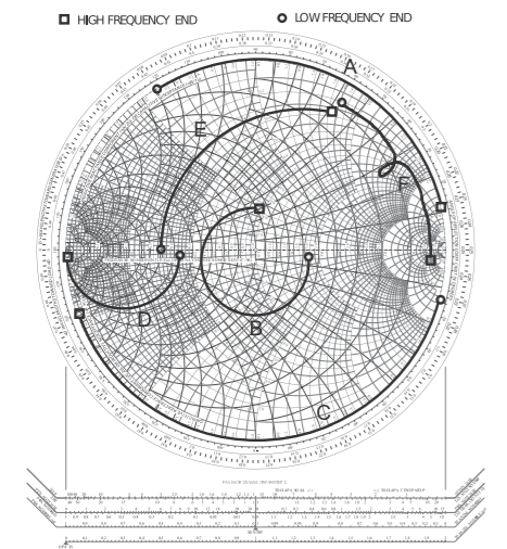
Figure \(\PageIndex{1}\): The locus of various loads plotted on a Smith chart.

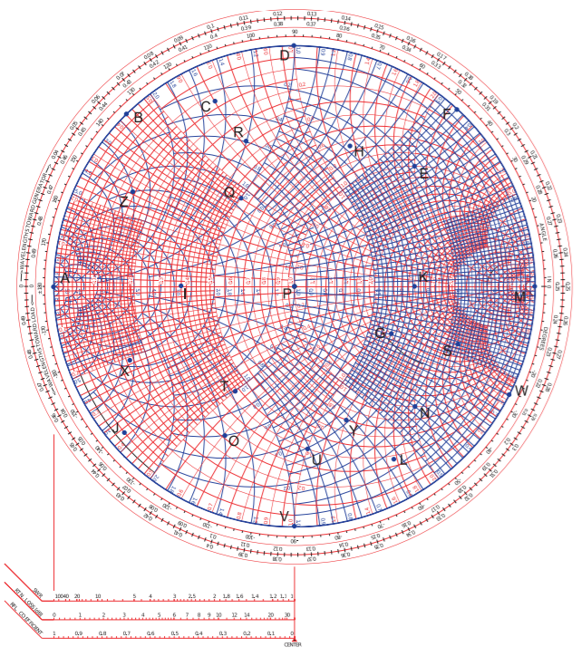
Figure \(\PageIndex{2}\)