3.1: Procedure

In previous work we have examined the basic functionality of Multisim, namely basic schematic capture functions such as component selection, placement, and parameter editing, along with simple simulations using virtual instruments such as a Digital Multimeter (DMM) to measure DC voltage. While virtual instruments are quick and easy to use, and offer some amount of familiarity, they are necessarily limited in other aspects. Some of the issues with virtual instruments include:

1. Limited measurements per unit, for example a single measurement for a DMM, requiring multiple units for multiple measurements.

2. The need to rewire the instruments (and hence the schematic) in order to take different readings.

3. Excessive amount of work space area obscured by the instrument(s) with accompanying clutter.

4. No convenient way of storing and recalling prior simulations.

5. No convenient means of exporting simulated measurement data to other programs.

To address these issues Multisim allows non-instrument simulations through the use of the Grapher window. The Grapher is a single, general purpose window that presents simulation data in both text and graphical form, as appropriate. Large amounts of data may be displayed simultaneously. The display itself is highly customizable (titles, axis ranges, colors, fonts, etc.). Each simulation is given its own sheet or tab and these may be saved for future reference. To top it off, nothing needs to be wired into the existing schematic and the Grapher may be minimized for greatest access to the schematic. The Grapher may be used for both DC and AC simulations, and includes interactive measurement tools for certain simulation types.

Because nothing is wired to the schematic, some means of identifying the measurement points is required. Multisim, like virtually all other simulation programs, does this through the use of numbered nodes. A node is simply a connection point in the circuit. Ground is always node number 0. The numbers increase as connections are made. Consequently, if the same circuit is entered by two different people who wire the components in a different order, the node numbers will not be the same between the two circuits. This is generally not a problem. As a side note, Multisim will not back-fill nodes that have been deleted. For example, if a circuit has been wired up to node ten and then node five is deleted, the next node to be wired will be numbered eleven, not five. Node number five will simply remain unused. Again, this is not a problem. It is important to note that, internally, Multisim always refers to connections via their node numbers, whether you use them or not.

When using virtual instruments, node numbers can add a certain amount of clutter to the schematic, consequently they are not shown by default. To show node numbers, select Sheet Properties from the Options menu. The dialog box of Figure \(\PageIndex{1}\) opens. This dialog box should be familiar as it was used in the prior exercise to set schematic colors and the like.

If the dialog box looks a little different from Figure \(\PageIndex{1}\), make sure that the Sheet Visibility tab is selected (leftmost tab). The center area is labeled Net Names. This controls whether or not node numbers will be visible on the schematic. To make node numbers visible, select Show All. Select OK to close the dialog box. We will now proceed to create a simple schematic.

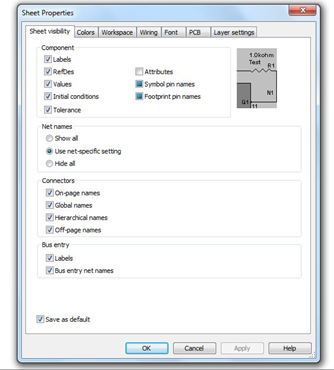
Figure \(\PageIndex{1}\)

Using virtual components, drag a DC voltage source, an earth ground and two resistors onto the work space. Connect them in a series loop and edit the component values to 20 volts for the source and 4000 and 6000 ohms for the two resistors. Once completed, the circuit should look something like Figure \(\PageIndex{2}\).

Note that ground is node zero. This is always the case. If the components were wired from left to right, the other two nodes will be one and two as shown. If the wiring steps were reversed, the node numbers will be reversed.

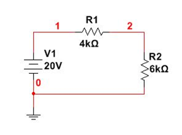
Figure \(\PageIndex{2}\)

We shall perform a simulation to inspect a few DC voltages. Instead of wiring in virtual DMMs, we shall select the Analyses and Simulation item under the Simulate menu (see Figure \(\PageIndex{3}\)).

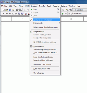
Figure \(\PageIndex{3}\)

A dialog box will open (see Figure \(\PageIndex{4}\)). There are well over a dozen analyses available. To find DC voltages or currents in our circuit, select DC Operating Point from the Analysis list. The dialog box will update and now contains two list areas. On the left will be a listing of available node voltages along with branch currents. The right side contains those items currently chosen for analysis. Node voltages will be shown with a V prefixed to the node number as in V(1). Branch currents will use an I prefix. In version 13 and earlier of Multisim the Analyses menu has a sub-menu of analysis choices. Simply select the analysis type from the sub-menu and then continue with the settings as described.

Select both nodes one and two on the input list with the mouse. To transfer them to the output list, select the Add button between the two lists. For now, this is all we need to concern ourselves with but it is worth mentioning that it is possible to create mathematical expressions of variables as well. For example, one node voltage could be subtracted from another in order to find the voltage across a single component or a group of components. Further, a node voltage could be squared and divided by a circuit resistance to determine the power dissipation.

Select the Run button at the bottom of the dialog to start the simulation.

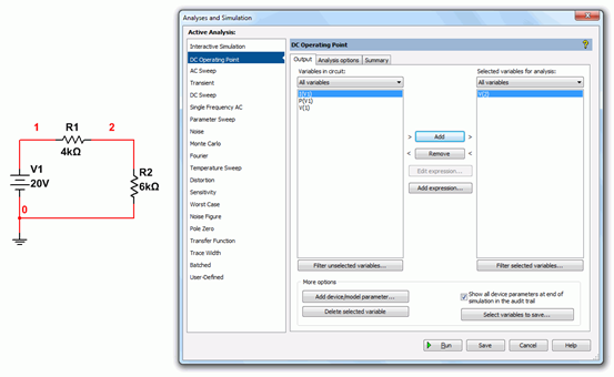
Figure \(\PageIndex{4}\)

After a moment, the Grapher window will appear as shown in Figure \(\PageIndex{5}\). For this simulation, the Grapher simply lists the node number and the corresponding voltage in two adjacent columns. This is a nice, compact display, much nicer than the individual DMM windows, especially if a large number of voltages are needed.

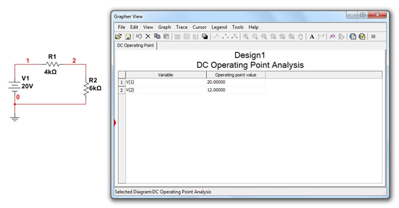
Figure \(\PageIndex{5}\)

Along the top of the Grapher window is a toolbar area for saving, cutting, customizing, and so forth. As useful as this is, the Grapher comes into its own when used with AC simulations.

Close the Grapher and modify the circuit to replace the DC source with an AC signal source as shown in Figure \(\PageIndex{6}\). Make sure that the new source is set to 20 volts with a frequency of 1000 Hz (1 kHz).

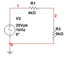
Figure \(\PageIndex{6}\)

We are going to examine the node voltages once again, however, this time the voltages will vary over time. If we were to use virtual instruments for this we’d choose once of the virtual oscilloscopes. In this case, however, we shall choose Transient Analysis from the Analyses and Simulation menu. A dialog box will open like that of Figure \(\PageIndex{7}\).

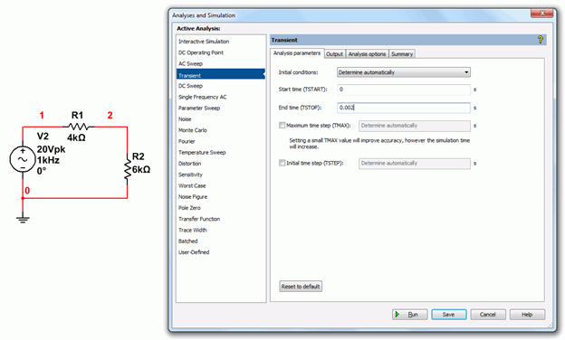
Figure \(\PageIndex{7}\)

The first thing we need to do is select the range of times we wish to see. Set the Start time to 0 and the End time to two milliseconds (0.002 seconds). Now select the Output tab. This is the same tab you saw back in Figure \(\PageIndex{4}\). Make sure that voltage nodes one and two are in the output analysis (right side) list. Now select Simulate. The Grapher will reopen with a display similar to that of Figure \(\PageIndex{8}\).

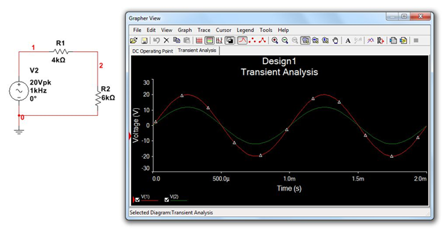
Figure \(\PageIndex{8}\)

The red and green traces graph the voltages at nodes one and two as they change through time. Note that there are many ways to customize this display. For example, selecting the white/black double square toward the middle of the toolbar will toggle the background color and labels between black and white. The grid pattern will overlay a measurement grid and the set of horizontal lines will bring up a color-node number legend. You can also click on the labels and axes to change them.

One of the more useful items is the pair of interactive cursors. The button for this is between the Legend and the Magnify buttons. Selecting this will bring up a pair of vertical cursors which may be grabbed and moved with the mouse. A separate cursor window will open. This will list the coordinates of the cursors on the plot lines along with the differences between the points (that is, how far apart the points are in time and in voltage). It will also list maxima and minima along with other useful data. An example of the Grapher with many of these settings in place is shown in Figure \(\PageIndex{9}\).

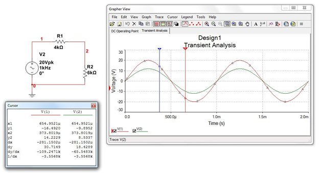
Figure \(\PageIndex{9}\)

Finally, note that the original DC Operating Point tab is still there. That is, you can quickly recall the original DC analysis by just selecting this tab. It should be clear by now that while the Grapher takes a little more to set up, it is far more flexible and useful than simple virtual instruments.