
4.3: Combining Parallel Components
- Page ID
- 25114

\( \newcommand{\vecs}[1]{\overset { \scriptstyle \rightharpoonup} {\mathbf{#1}} } \)
\( \newcommand{\vecd}[1]{\overset{-\!-\!\rightharpoonup}{\vphantom{a}\smash {#1}}} \)
\( \newcommand{\dsum}{\displaystyle\sum\limits} \)
\( \newcommand{\dint}{\displaystyle\int\limits} \)
\( \newcommand{\dlim}{\displaystyle\lim\limits} \)
\( \newcommand{\id}{\mathrm{id}}\) \( \newcommand{\Span}{\mathrm{span}}\)
( \newcommand{\kernel}{\mathrm{null}\,}\) \( \newcommand{\range}{\mathrm{range}\,}\)
\( \newcommand{\RealPart}{\mathrm{Re}}\) \( \newcommand{\ImaginaryPart}{\mathrm{Im}}\)
\( \newcommand{\Argument}{\mathrm{Arg}}\) \( \newcommand{\norm}[1]{\| #1 \|}\)
\( \newcommand{\inner}[2]{\langle #1, #2 \rangle}\)
\( \newcommand{\Span}{\mathrm{span}}\)
\( \newcommand{\id}{\mathrm{id}}\)
\( \newcommand{\Span}{\mathrm{span}}\)
\( \newcommand{\kernel}{\mathrm{null}\,}\)
\( \newcommand{\range}{\mathrm{range}\,}\)
\( \newcommand{\RealPart}{\mathrm{Re}}\)
\( \newcommand{\ImaginaryPart}{\mathrm{Im}}\)
\( \newcommand{\Argument}{\mathrm{Arg}}\)
\( \newcommand{\norm}[1]{\| #1 \|}\)
\( \newcommand{\inner}[2]{\langle #1, #2 \rangle}\)
\( \newcommand{\Span}{\mathrm{span}}\) \( \newcommand{\AA}{\unicode[.8,0]{x212B}}\)
\( \newcommand{\vectorA}[1]{\vec{#1}} % arrow\)
\( \newcommand{\vectorAt}[1]{\vec{\text{#1}}} % arrow\)
\( \newcommand{\vectorB}[1]{\overset { \scriptstyle \rightharpoonup} {\mathbf{#1}} } \)
\( \newcommand{\vectorC}[1]{\textbf{#1}} \)
\( \newcommand{\vectorD}[1]{\overrightarrow{#1}} \)
\( \newcommand{\vectorDt}[1]{\overrightarrow{\text{#1}}} \)
\( \newcommand{\vectE}[1]{\overset{-\!-\!\rightharpoonup}{\vphantom{a}\smash{\mathbf {#1}}}} \)
\( \newcommand{\vecs}[1]{\overset { \scriptstyle \rightharpoonup} {\mathbf{#1}} } \)
\(\newcommand{\longvect}{\overrightarrow}\)
\( \newcommand{\vecd}[1]{\overset{-\!-\!\rightharpoonup}{\vphantom{a}\smash {#1}}} \)
\(\newcommand{\avec}{\mathbf a}\) \(\newcommand{\bvec}{\mathbf b}\) \(\newcommand{\cvec}{\mathbf c}\) \(\newcommand{\dvec}{\mathbf d}\) \(\newcommand{\dtil}{\widetilde{\mathbf d}}\) \(\newcommand{\evec}{\mathbf e}\) \(\newcommand{\fvec}{\mathbf f}\) \(\newcommand{\nvec}{\mathbf n}\) \(\newcommand{\pvec}{\mathbf p}\) \(\newcommand{\qvec}{\mathbf q}\) \(\newcommand{\svec}{\mathbf s}\) \(\newcommand{\tvec}{\mathbf t}\) \(\newcommand{\uvec}{\mathbf u}\) \(\newcommand{\vvec}{\mathbf v}\) \(\newcommand{\wvec}{\mathbf w}\) \(\newcommand{\xvec}{\mathbf x}\) \(\newcommand{\yvec}{\mathbf y}\) \(\newcommand{\zvec}{\mathbf z}\) \(\newcommand{\rvec}{\mathbf r}\) \(\newcommand{\mvec}{\mathbf m}\) \(\newcommand{\zerovec}{\mathbf 0}\) \(\newcommand{\onevec}{\mathbf 1}\) \(\newcommand{\real}{\mathbb R}\) \(\newcommand{\twovec}[2]{\left[\begin{array}{r}#1 \\ #2 \end{array}\right]}\) \(\newcommand{\ctwovec}[2]{\left[\begin{array}{c}#1 \\ #2 \end{array}\right]}\) \(\newcommand{\threevec}[3]{\left[\begin{array}{r}#1 \\ #2 \\ #3 \end{array}\right]}\) \(\newcommand{\cthreevec}[3]{\left[\begin{array}{c}#1 \\ #2 \\ #3 \end{array}\right]}\) \(\newcommand{\fourvec}[4]{\left[\begin{array}{r}#1 \\ #2 \\ #3 \\ #4 \end{array}\right]}\) \(\newcommand{\cfourvec}[4]{\left[\begin{array}{c}#1 \\ #2 \\ #3 \\ #4 \end{array}\right]}\) \(\newcommand{\fivevec}[5]{\left[\begin{array}{r}#1 \\ #2 \\ #3 \\ #4 \\ #5 \\ \end{array}\right]}\) \(\newcommand{\cfivevec}[5]{\left[\begin{array}{c}#1 \\ #2 \\ #3 \\ #4 \\ #5 \\ \end{array}\right]}\) \(\newcommand{\mattwo}[4]{\left[\begin{array}{rr}#1 \amp #2 \\ #3 \amp #4 \\ \end{array}\right]}\) \(\newcommand{\laspan}[1]{\text{Span}\{#1\}}\) \(\newcommand{\bcal}{\cal B}\) \(\newcommand{\ccal}{\cal C}\) \(\newcommand{\scal}{\cal S}\) \(\newcommand{\wcal}{\cal W}\) \(\newcommand{\ecal}{\cal E}\) \(\newcommand{\coords}[2]{\left\{#1\right\}_{#2}}\) \(\newcommand{\gray}[1]{\color{gray}{#1}}\) \(\newcommand{\lgray}[1]{\color{lightgray}{#1}}\) \(\newcommand{\rank}{\operatorname{rank}}\) \(\newcommand{\row}{\text{Row}}\) \(\newcommand{\col}{\text{Col}}\) \(\renewcommand{\row}{\text{Row}}\) \(\newcommand{\nul}{\text{Nul}}\) \(\newcommand{\var}{\text{Var}}\) \(\newcommand{\corr}{\text{corr}}\) \(\newcommand{\len}[1]{\left|#1\right|}\) \(\newcommand{\bbar}{\overline{\bvec}}\) \(\newcommand{\bhat}{\widehat{\bvec}}\) \(\newcommand{\bperp}{\bvec^\perp}\) \(\newcommand{\xhat}{\widehat{\xvec}}\) \(\newcommand{\vhat}{\widehat{\vvec}}\) \(\newcommand{\uhat}{\widehat{\uvec}}\) \(\newcommand{\what}{\widehat{\wvec}}\) \(\newcommand{\Sighat}{\widehat{\Sigma}}\) \(\newcommand{\lt}{<}\) \(\newcommand{\gt}{>}\) \(\newcommand{\amp}{&}\) \(\definecolor{fillinmathshade}{gray}{0.9}\)Our first step is to determine how to combine parallel components in order to create a single equivalent component. Unlike series connections, this can be a little more time consuming.
Sources in Parallel
First, voltage sources are not placed in parallel as a general rule, see Figure 4.3.1 . The reason is because a parallel connection requires the same voltage across each component. This would be impossible to achieve with each source trying to maintain a different voltage across the same two nodes. This may result in damage to the sources (e.g., exploding batteries). The main exception to this rule is if the sources have the same potential and the goal is to extend operational life (e.g., multiple D cell batteries in parallel).
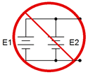
Figure 4.3.1 : Do not place voltage sources in parallel.
When it comes to current sources, they may simply be added together, however, like series voltage sources, polarity is important. Referring to the three parallel current sources in Figure 4.3.2 , the middle and right sources are pumping current into the top node while the left source is feeding the bottom node. You can also think of the left source as draining the top node. Thus, these three sources together behave like a single source of five amps feeding the top node (eight amps in, three amps out).
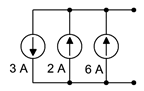
Figure 4.3.2 : Current sources in parallel.
Resistors in Parallel
When placed in parallel, resistor values do not add they way they do in series connections. The reason for this is obvious if we look at the basic resistance equation from Chapter 2, Equation 2.11:
\[R = \frac{\rho l}{A} \nonumber \]
If we consider two identical resistors placed in parallel, side by side as in Figure 4.3.3 , the effective area would double while keeping the resistivity and length unchanged. The combined result would be a halving of the resistance of just one of them. Thus we see that placing resistors in parallel results in a decrease in net resistance, the opposite of the series case.
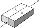
Figure 4.3.3 : Resistors in parallel.
This situation is simplified if we consider conductance instead of resistance. Recalling that conductance, G, is the reciprocal of resistance, we can rewrite the resistance equation:
\[G = \frac{A}{\rho l} \nonumber \]
Now we can see that the increase in area creates a proportional increase in conductivity. If we generalize this for \(N\) resistors we find that the equivalent conductance of a group of parallel resistors is their sum:
\[G_{Total} = G_1+G_2+G_3+ \dots +G_N \label{4.2} \]
As we deal normally with component resistance values instead of conductance values, Equation \ref{4.2} may be rewritten in terms of equivalent resistance:
\[\frac{1}{R_{Parallel}} = \frac{1}{R_1} + \frac{1}{R_2} + \frac{1}{R_3} + \dots + \frac{1}{R_N} \\ R_{Parallel} = \frac{1}{\frac{1}{R_1} + \frac{1}{R_2} + \frac{1}{R_3} + \dots + \frac{1}{R_N}} \label{4.3} \]
Among other things, Equation \ref{4.3} tells us that the equivalent resistance of a group of parallel resistances will always be smaller than the smallest resistance in that group. It also indicates that if we have \(N\) identical resistors of value \(R\), the equivalent will be \(R/N\) (e.g., 3 parallel 3.6 k\( \Omega \) resistors are equivalent to a single 1.2 k\( \Omega \) resistor). As a convenience, it is common to use two parallel lines, \(||\), as a shortcut way of saying “in parallel with”, as in \(R_1 || R_2\). Also, \(||\) has higher operational precedence than +.
Product-Sum Rule
A handy shortcut for two parallel resistors may be created from Equation \ref{4.3}. We start by writing the version for just two parallel resistors,
\[R_{Parallel} = \frac{1}{\frac{1}{R_1} + \frac{1}{R_2}} \nonumber \]
Multiply the fraction through by \(R_1\) \(R_2\) and simplify:
\[R_{Parallel} = \frac{R_1 R_2}{R_1+R_2} \label{4.4} \]
For obvious reasons, Equation \ref{4.4} is referred to as the product-sum rule. It is only applicable to two resistors, however, it can be used repeatedly on pairs of resistors within larger groups instead of using Equation \ref{4.3}. For example, a group of four resistors can be reduced to two pairs, and then those two equivalents can be reduced as a third pair. This can be a handy technique for obtaining quick estimates.
We can take the product-sum rule a step further by writing \(R_2\) as a multiple of \(R_1\):
\[R_2 = N R_1 \nonumber \]
Substituting this into Equation \ref{4.4} yields:
\[R_{Parallel} = \frac{R_1 N R_1}{R_1+N R_1} \nonumber \]
\[R_{Parallel} = \frac{N R_1^2}{(N+1)R_1} \nonumber \]
\[R_{Parallel} = \frac{N}{N+1} R_1 \label{4.5} \]
Equation \ref{4.5} is useful for quick estimates of parallel resistor pairs. For example, if we have a 24 k\( \Omega \) resistor in parallel with an 8 k\( \Omega \) resistor, that's a ratio (\(N\)) of 3:1. Thus the equivalent will be \(N/(N+1)\), or 3/4ths, of the smaller resistor, yielding 6 k\( \Omega \). Similarly, a 180 \( \Omega \) in parallel with a 90 \( \Omega \) would yield 2/3rds of 90 \( \Omega \), or 60 \( \Omega \).
A group of resistors is placed in parallel as shown in Figure 4.3.4 . Determine the equivalent parallel value.
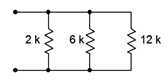
Figure 4.3.4 : Resistor arrangement for Example 4.3.1 .
There are several solution paths. We'll try them all and compare. First, let's try the conductance form:
\[R_{Parallel} = \frac{1}{\frac{1}{R_1} + \frac{1}{R_2} + \frac{1}{R_3} + \dots + \frac{1}{R_N}} \nonumber \]
\[R_{Parallel} = \frac{1}{\frac{1}{2k \Omega } + \frac{1}{6k \Omega } + \frac{1}{12 k \Omega }} \nonumber \]
\[R_{Parallel} \approx 1.333 k \Omega \nonumber \]
We could also use the product-sum rule twice. We'll use the middle and right-most resistor first (although any pairing would do, but this pairing is convenient):
\[R_{23} = \frac{R_2 R_3}{R_2+R_3} \nonumber \]
\[R_{23} = \frac{6k \Omega 12 k \Omega }{6 k \Omega +12k \Omega } \nonumber \]
\[R_{23} = 4 k \Omega \nonumber \]
\[R_{Parallel} = \frac{R_1 R_{23}}{R_1+R_{23}} \nonumber \]
\[R_{Parallel} = \frac{2 k \Omega 4 k \Omega }{2 k \Omega +4k \Omega } \nonumber \]
\[R_{Parallel} \approx 1.333 k \Omega \nonumber \]
Finally, we could use the ratio technique. First, consider the 6 k\( \Omega \) and 12 k\( \Omega \) resistor pair. That's a 2:1 ratio, so the result will be 2/3rds of the smaller resistor, and 2/3rds of 6 k\( \Omega \) is 4 k\( \Omega \). The ratio between this and the 2 k\( \Omega \) resistor is also 2:1, and 2/3rds of 2 k\( \Omega \) is approximately 1.333 k\( \Omega \).
The ratio technique happened to work out well here because of the convenient resistor values with perfect integer ratios. That will not always be the case.