
6.3: Superposition Theorem
- Page ID
- 25128

\( \newcommand{\vecs}[1]{\overset { \scriptstyle \rightharpoonup} {\mathbf{#1}} } \)
\( \newcommand{\vecd}[1]{\overset{-\!-\!\rightharpoonup}{\vphantom{a}\smash {#1}}} \)
\( \newcommand{\dsum}{\displaystyle\sum\limits} \)
\( \newcommand{\dint}{\displaystyle\int\limits} \)
\( \newcommand{\dlim}{\displaystyle\lim\limits} \)
\( \newcommand{\id}{\mathrm{id}}\) \( \newcommand{\Span}{\mathrm{span}}\)
( \newcommand{\kernel}{\mathrm{null}\,}\) \( \newcommand{\range}{\mathrm{range}\,}\)
\( \newcommand{\RealPart}{\mathrm{Re}}\) \( \newcommand{\ImaginaryPart}{\mathrm{Im}}\)
\( \newcommand{\Argument}{\mathrm{Arg}}\) \( \newcommand{\norm}[1]{\| #1 \|}\)
\( \newcommand{\inner}[2]{\langle #1, #2 \rangle}\)
\( \newcommand{\Span}{\mathrm{span}}\)
\( \newcommand{\id}{\mathrm{id}}\)
\( \newcommand{\Span}{\mathrm{span}}\)
\( \newcommand{\kernel}{\mathrm{null}\,}\)
\( \newcommand{\range}{\mathrm{range}\,}\)
\( \newcommand{\RealPart}{\mathrm{Re}}\)
\( \newcommand{\ImaginaryPart}{\mathrm{Im}}\)
\( \newcommand{\Argument}{\mathrm{Arg}}\)
\( \newcommand{\norm}[1]{\| #1 \|}\)
\( \newcommand{\inner}[2]{\langle #1, #2 \rangle}\)
\( \newcommand{\Span}{\mathrm{span}}\) \( \newcommand{\AA}{\unicode[.8,0]{x212B}}\)
\( \newcommand{\vectorA}[1]{\vec{#1}} % arrow\)
\( \newcommand{\vectorAt}[1]{\vec{\text{#1}}} % arrow\)
\( \newcommand{\vectorB}[1]{\overset { \scriptstyle \rightharpoonup} {\mathbf{#1}} } \)
\( \newcommand{\vectorC}[1]{\textbf{#1}} \)
\( \newcommand{\vectorD}[1]{\overrightarrow{#1}} \)
\( \newcommand{\vectorDt}[1]{\overrightarrow{\text{#1}}} \)
\( \newcommand{\vectE}[1]{\overset{-\!-\!\rightharpoonup}{\vphantom{a}\smash{\mathbf {#1}}}} \)
\( \newcommand{\vecs}[1]{\overset { \scriptstyle \rightharpoonup} {\mathbf{#1}} } \)
\( \newcommand{\vecd}[1]{\overset{-\!-\!\rightharpoonup}{\vphantom{a}\smash {#1}}} \)
\(\newcommand{\avec}{\mathbf a}\) \(\newcommand{\bvec}{\mathbf b}\) \(\newcommand{\cvec}{\mathbf c}\) \(\newcommand{\dvec}{\mathbf d}\) \(\newcommand{\dtil}{\widetilde{\mathbf d}}\) \(\newcommand{\evec}{\mathbf e}\) \(\newcommand{\fvec}{\mathbf f}\) \(\newcommand{\nvec}{\mathbf n}\) \(\newcommand{\pvec}{\mathbf p}\) \(\newcommand{\qvec}{\mathbf q}\) \(\newcommand{\svec}{\mathbf s}\) \(\newcommand{\tvec}{\mathbf t}\) \(\newcommand{\uvec}{\mathbf u}\) \(\newcommand{\vvec}{\mathbf v}\) \(\newcommand{\wvec}{\mathbf w}\) \(\newcommand{\xvec}{\mathbf x}\) \(\newcommand{\yvec}{\mathbf y}\) \(\newcommand{\zvec}{\mathbf z}\) \(\newcommand{\rvec}{\mathbf r}\) \(\newcommand{\mvec}{\mathbf m}\) \(\newcommand{\zerovec}{\mathbf 0}\) \(\newcommand{\onevec}{\mathbf 1}\) \(\newcommand{\real}{\mathbb R}\) \(\newcommand{\twovec}[2]{\left[\begin{array}{r}#1 \\ #2 \end{array}\right]}\) \(\newcommand{\ctwovec}[2]{\left[\begin{array}{c}#1 \\ #2 \end{array}\right]}\) \(\newcommand{\threevec}[3]{\left[\begin{array}{r}#1 \\ #2 \\ #3 \end{array}\right]}\) \(\newcommand{\cthreevec}[3]{\left[\begin{array}{c}#1 \\ #2 \\ #3 \end{array}\right]}\) \(\newcommand{\fourvec}[4]{\left[\begin{array}{r}#1 \\ #2 \\ #3 \\ #4 \end{array}\right]}\) \(\newcommand{\cfourvec}[4]{\left[\begin{array}{c}#1 \\ #2 \\ #3 \\ #4 \end{array}\right]}\) \(\newcommand{\fivevec}[5]{\left[\begin{array}{r}#1 \\ #2 \\ #3 \\ #4 \\ #5 \\ \end{array}\right]}\) \(\newcommand{\cfivevec}[5]{\left[\begin{array}{c}#1 \\ #2 \\ #3 \\ #4 \\ #5 \\ \end{array}\right]}\) \(\newcommand{\mattwo}[4]{\left[\begin{array}{rr}#1 \amp #2 \\ #3 \amp #4 \\ \end{array}\right]}\) \(\newcommand{\laspan}[1]{\text{Span}\{#1\}}\) \(\newcommand{\bcal}{\cal B}\) \(\newcommand{\ccal}{\cal C}\) \(\newcommand{\scal}{\cal S}\) \(\newcommand{\wcal}{\cal W}\) \(\newcommand{\ecal}{\cal E}\) \(\newcommand{\coords}[2]{\left\{#1\right\}_{#2}}\) \(\newcommand{\gray}[1]{\color{gray}{#1}}\) \(\newcommand{\lgray}[1]{\color{lightgray}{#1}}\) \(\newcommand{\rank}{\operatorname{rank}}\) \(\newcommand{\row}{\text{Row}}\) \(\newcommand{\col}{\text{Col}}\) \(\renewcommand{\row}{\text{Row}}\) \(\newcommand{\nul}{\text{Nul}}\) \(\newcommand{\var}{\text{Var}}\) \(\newcommand{\corr}{\text{corr}}\) \(\newcommand{\len}[1]{\left|#1\right|}\) \(\newcommand{\bbar}{\overline{\bvec}}\) \(\newcommand{\bhat}{\widehat{\bvec}}\) \(\newcommand{\bperp}{\bvec^\perp}\) \(\newcommand{\xhat}{\widehat{\xvec}}\) \(\newcommand{\vhat}{\widehat{\vvec}}\) \(\newcommand{\uhat}{\widehat{\uvec}}\) \(\newcommand{\what}{\widehat{\wvec}}\) \(\newcommand{\Sighat}{\widehat{\Sigma}}\) \(\newcommand{\lt}{<}\) \(\newcommand{\gt}{>}\) \(\newcommand{\amp}{&}\) \(\definecolor{fillinmathshade}{gray}{0.9}\)As useful as the source conversion technique proved to be in Example 6.2.3, it will not work for all circuits. Thus, more general approaches are needed. One of these methods is superposition.
Superposition allows the analysis of multi-source series-parallel circuits. Superposition can only be applied to networks that are linear and bilateral. Further, it cannot be used to find values for non-linear functions, such as power, directly. Fortunately, if the circuit contains nothing but resistors, and ordinary voltage sources and current sources, the circuit will be a linear bilateral network. Also, although power is a square law function (i.e., it is proportional to the square of voltage or current), it can be computed from the resulting voltage or current values so this presents no limits to analysis.
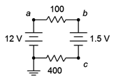
Figure 6.3.1 : A dual source circuit.
The basic idea is to determine the contribution of each source by itself, and then adding the results to get the final answer(s). Let's start with an almost trivial example to illustrate the idea. Consider the circuit of Figure 6.3.1 . Here we have two voltage sources driving a pair of resistors. It is a basic series circuit. The way this was approached in Chapter 3 was to combine the sources and the resistors into a single source and resistor. The circulating current could then be found using Ohm's law. As the two sources are in opposition, the net voltage is 10.5 volts while the total resistance is 500 \(\Omega\). This yields a circulating current of 21 mA.
Instead of this approach, let's consider the contribution of each source by itself. To do that, we will replace all other sources in the circuit with their ideal internal resistance. From earlier work we have discovered that the ideal internal resistance of a voltage source is a short, or zero ohms. Thus, we wind up with two circuits: one with a 12 volt source that drives 100 \(\Omega\), 400 \(\Omega\) and a short; and a second circuit with a 1.5 volt source that drives pretty much the same thing, but with an opposing current direction. The first circuit produces a clockwise current of 12 V/ 500 \(\Omega\), or 24 milliamps. Meanwhile, the second circuit produces a counterclockwise current of 1.5 V / 500 \(\Omega\), or 3 mA. As these two currents oppose each other, the resulting current is 24 mA − 3 mA, or 21 mA, the same value originally computed. Granted, this second method is less efficient than the original method but it illustrates the process. More importantly, this process can be applied to a variety of multi-source series-parallel circuits. A key element is to remember the directions of the currents and polarities of the voltages created in the sub-circuits. Without these data, it will be impossible to determine whether the various pieces of the puzzle are added to or subtracted from the total.
To summarize the superposition technique:
- For every voltage or current source in the original circuit, create a new subcircuit. The sub-circuits will be identical to the original except that all sources other than the one under consideration will be replaced by their ideal internal resistance. This means that all remaining voltage sources will be shorted and all remaining current sources will be opened.
- Label the current directions and voltage polarities on each of the new subcircuits, as generated by the source under consideration.
- Solve each of the sub-circuits for the desired voltages and/or currents using standard series-parallel analysis techniques. Make sure to note the voltage polarities and current directions for these items.
- Add all of the contributions from each of the sub-circuits to arrive at the final values, being sure to account for current directions and voltage polarities in the process.
In order to get a better handle on the superposition technique, let's reexamine the the dual source circuit shown in Figure 6.2.8 (repeated in Figure 6.3.2 for ease of reference). We will solve this using superposition. As the circuit has two sources, it will require two sub-circuits.
Determine \(V_b\) for the circuit of Figure 6.3.2 using superposition.
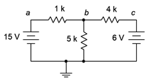
Figure 6.3.2 : Circuit for Example 6.3.1 .
As this circuit has two voltage sources, two sub-circuits will be needed. The first sub-circuit will use the 15 volt source. Consequently, the 6 volt source will be replaced with its ideal internal resistance, a short. This new circuit is shown in Figure 6.3.3 .
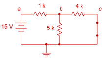
Figure 6.3.3 : First sub-circuit for the circuit of Figure 6.3.2 .
The current directions are as follows: current exits the source and travels through the 1 k\(\Omega\) producing a voltage drop + to − from left to right. At node \(b\) the current splits. The 4 k\(\Omega\) and 5 k\(\Omega\) are in parallel so they both see the same voltage. Some of the current flows down through the 5 k\(\Omega\) resistor producing a voltage drop + to − from top to bottom. The remainder of the current flows to the right, through the 4 k\(\Omega\), producing a voltage drop + to − from left to right. \(V_b\) can be determined via voltage divider between the 1 k\(\Omega\) and the parallel combo of the 5 k\(\Omega\) and 4 k\(\Omega\). 5 k\(\Omega\) in parallel with 4 k\(\Omega\) is approximately 2.222 k\(\Omega\).
\[V_b = E \frac{R_x}{R_x+R_y} \nonumber \]
\[V_b = 15V \frac{2.222 k \Omega}{2.222 k\Omega +1 k\Omega} \nonumber \]
\[V_b \approx 10.34 V \nonumber \]
The second sub-circuit will use the 6 volt source. Therefore, the 15 volt source will be replaced with its ideal internal resistance, a short. This new circuit is shown in Figure 6.3.4 .
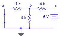
Figure 6.3.4 : Second sub-circuit for the circuit of Figure 6.3.2 .
The current directions are as follows: current exits the source and travels through the 4 k\(\Omega\) producing a voltage drop + to − from right to left. At node \(b\) the current splits. Now the 1 k\(\Omega\) and 5 k\(\Omega\) are in parallel so they both see the same voltage. Some of the current flows down through the 5 k\(\Omega\) resistor producing a voltage drop + to − from top to bottom, just as it did in the first sub-circuit. The remainder of the current flows to the left, through the 1 k\(\Omega\), producing a voltage drop + to − from right to left. Once again, \(V_b\) can be determined via voltage divider, this time between the 4 k\(\Omega\) and the parallel combo of the 5 k\(\Omega\) and 1 k\(\Omega\) is approximately 833.3 \(\Omega\).
\[V_b = E \frac{R_x}{R_x+R_y} \nonumber \]
\[V_b = 6V \frac{833.3\Omega}{833.3\Omega +4 k\Omega} \nonumber \]
\[V_b \approx 1.034 V \nonumber \]
Both sub-circuits show polarities of + to − from top to bottom for \(V_b\), therefore these two voltages simply add, for a total of approximately 11.37 volts. This agrees nicely with the result obtained using source conversions. The slight deviation in the final digit is no doubt due to the rounding of intermediate values, such as resistor combinations.
It is instructive to pursue this example further and investigate a current. In the source conversion version it was discovered that the current through the 1 k\(\Omega\) resistor is 3.62 mA and flowing left to right. Using superposition, the corresponding current in the first sub-circuit can be found using KVL and Ohm's law, (15 V − 10.34 V)/ 1 k\(\Omega\), or 4.66 mA flowing left to right. In the second sub-circuit, this current can be obtained using Ohm's law alone, 1.034 V / 1 k\(\Omega\), or 1.034 mA flowing right to left. As this current opposes the current from the first sub-circuit, the two values are subtracting leaving approximately 3.63 mA flowing left to right, agreeing with the original answer within rounding error.
Computer Simulation
For further verification, the circuit of Example 6.3.1 is entered into a simulator as shown in Figure 6.3.5 .
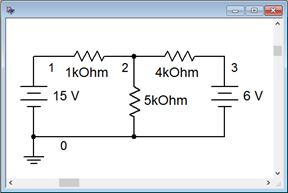
Figure 6.3.5 : The circuit of Example 6.3.1 in a simulator.
A DC operating point analysis is performed, as shown in Figure 6.3.6 .
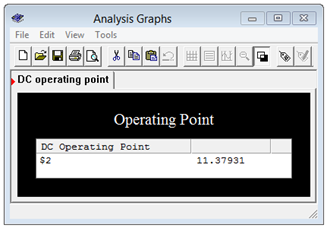
Figure 6.3.6 : Simulation results for the circuit of Example 6.3.1 .
The voltage at node 2, which is \(V_b\) in the original circuit, agrees nicely with the values computed previously.
This exploration shows that the superposition technique offers a fairly straightforward method of solving a variety of multi-source series-parallel circuits. It is not without its limitations, though. First, if a circuit has a large number of sources, superposition can become a bit tedious as it requires as many sub-circuits as there are sources, and every one of these sub-circuits requires separate solutions. Second, there are some series-parallel configurations that superposition along with seriesparallel analysis techniques will not solve. We will investigate methods of dealing with these issues later in this chapter and in the following chapter.