
8.4: Transient Response of RC Circuits
- Page ID
- 25143

\( \newcommand{\vecs}[1]{\overset { \scriptstyle \rightharpoonup} {\mathbf{#1}} } \)
\( \newcommand{\vecd}[1]{\overset{-\!-\!\rightharpoonup}{\vphantom{a}\smash {#1}}} \)
\( \newcommand{\dsum}{\displaystyle\sum\limits} \)
\( \newcommand{\dint}{\displaystyle\int\limits} \)
\( \newcommand{\dlim}{\displaystyle\lim\limits} \)
\( \newcommand{\id}{\mathrm{id}}\) \( \newcommand{\Span}{\mathrm{span}}\)
( \newcommand{\kernel}{\mathrm{null}\,}\) \( \newcommand{\range}{\mathrm{range}\,}\)
\( \newcommand{\RealPart}{\mathrm{Re}}\) \( \newcommand{\ImaginaryPart}{\mathrm{Im}}\)
\( \newcommand{\Argument}{\mathrm{Arg}}\) \( \newcommand{\norm}[1]{\| #1 \|}\)
\( \newcommand{\inner}[2]{\langle #1, #2 \rangle}\)
\( \newcommand{\Span}{\mathrm{span}}\)
\( \newcommand{\id}{\mathrm{id}}\)
\( \newcommand{\Span}{\mathrm{span}}\)
\( \newcommand{\kernel}{\mathrm{null}\,}\)
\( \newcommand{\range}{\mathrm{range}\,}\)
\( \newcommand{\RealPart}{\mathrm{Re}}\)
\( \newcommand{\ImaginaryPart}{\mathrm{Im}}\)
\( \newcommand{\Argument}{\mathrm{Arg}}\)
\( \newcommand{\norm}[1]{\| #1 \|}\)
\( \newcommand{\inner}[2]{\langle #1, #2 \rangle}\)
\( \newcommand{\Span}{\mathrm{span}}\) \( \newcommand{\AA}{\unicode[.8,0]{x212B}}\)
\( \newcommand{\vectorA}[1]{\vec{#1}} % arrow\)
\( \newcommand{\vectorAt}[1]{\vec{\text{#1}}} % arrow\)
\( \newcommand{\vectorB}[1]{\overset { \scriptstyle \rightharpoonup} {\mathbf{#1}} } \)
\( \newcommand{\vectorC}[1]{\textbf{#1}} \)
\( \newcommand{\vectorD}[1]{\overrightarrow{#1}} \)
\( \newcommand{\vectorDt}[1]{\overrightarrow{\text{#1}}} \)
\( \newcommand{\vectE}[1]{\overset{-\!-\!\rightharpoonup}{\vphantom{a}\smash{\mathbf {#1}}}} \)
\( \newcommand{\vecs}[1]{\overset { \scriptstyle \rightharpoonup} {\mathbf{#1}} } \)
\( \newcommand{\vecd}[1]{\overset{-\!-\!\rightharpoonup}{\vphantom{a}\smash {#1}}} \)
\(\newcommand{\avec}{\mathbf a}\) \(\newcommand{\bvec}{\mathbf b}\) \(\newcommand{\cvec}{\mathbf c}\) \(\newcommand{\dvec}{\mathbf d}\) \(\newcommand{\dtil}{\widetilde{\mathbf d}}\) \(\newcommand{\evec}{\mathbf e}\) \(\newcommand{\fvec}{\mathbf f}\) \(\newcommand{\nvec}{\mathbf n}\) \(\newcommand{\pvec}{\mathbf p}\) \(\newcommand{\qvec}{\mathbf q}\) \(\newcommand{\svec}{\mathbf s}\) \(\newcommand{\tvec}{\mathbf t}\) \(\newcommand{\uvec}{\mathbf u}\) \(\newcommand{\vvec}{\mathbf v}\) \(\newcommand{\wvec}{\mathbf w}\) \(\newcommand{\xvec}{\mathbf x}\) \(\newcommand{\yvec}{\mathbf y}\) \(\newcommand{\zvec}{\mathbf z}\) \(\newcommand{\rvec}{\mathbf r}\) \(\newcommand{\mvec}{\mathbf m}\) \(\newcommand{\zerovec}{\mathbf 0}\) \(\newcommand{\onevec}{\mathbf 1}\) \(\newcommand{\real}{\mathbb R}\) \(\newcommand{\twovec}[2]{\left[\begin{array}{r}#1 \\ #2 \end{array}\right]}\) \(\newcommand{\ctwovec}[2]{\left[\begin{array}{c}#1 \\ #2 \end{array}\right]}\) \(\newcommand{\threevec}[3]{\left[\begin{array}{r}#1 \\ #2 \\ #3 \end{array}\right]}\) \(\newcommand{\cthreevec}[3]{\left[\begin{array}{c}#1 \\ #2 \\ #3 \end{array}\right]}\) \(\newcommand{\fourvec}[4]{\left[\begin{array}{r}#1 \\ #2 \\ #3 \\ #4 \end{array}\right]}\) \(\newcommand{\cfourvec}[4]{\left[\begin{array}{c}#1 \\ #2 \\ #3 \\ #4 \end{array}\right]}\) \(\newcommand{\fivevec}[5]{\left[\begin{array}{r}#1 \\ #2 \\ #3 \\ #4 \\ #5 \\ \end{array}\right]}\) \(\newcommand{\cfivevec}[5]{\left[\begin{array}{c}#1 \\ #2 \\ #3 \\ #4 \\ #5 \\ \end{array}\right]}\) \(\newcommand{\mattwo}[4]{\left[\begin{array}{rr}#1 \amp #2 \\ #3 \amp #4 \\ \end{array}\right]}\) \(\newcommand{\laspan}[1]{\text{Span}\{#1\}}\) \(\newcommand{\bcal}{\cal B}\) \(\newcommand{\ccal}{\cal C}\) \(\newcommand{\scal}{\cal S}\) \(\newcommand{\wcal}{\cal W}\) \(\newcommand{\ecal}{\cal E}\) \(\newcommand{\coords}[2]{\left\{#1\right\}_{#2}}\) \(\newcommand{\gray}[1]{\color{gray}{#1}}\) \(\newcommand{\lgray}[1]{\color{lightgray}{#1}}\) \(\newcommand{\rank}{\operatorname{rank}}\) \(\newcommand{\row}{\text{Row}}\) \(\newcommand{\col}{\text{Col}}\) \(\renewcommand{\row}{\text{Row}}\) \(\newcommand{\nul}{\text{Nul}}\) \(\newcommand{\var}{\text{Var}}\) \(\newcommand{\corr}{\text{corr}}\) \(\newcommand{\len}[1]{\left|#1\right|}\) \(\newcommand{\bbar}{\overline{\bvec}}\) \(\newcommand{\bhat}{\widehat{\bvec}}\) \(\newcommand{\bperp}{\bvec^\perp}\) \(\newcommand{\xhat}{\widehat{\xvec}}\) \(\newcommand{\vhat}{\widehat{\vvec}}\) \(\newcommand{\uhat}{\widehat{\uvec}}\) \(\newcommand{\what}{\widehat{\wvec}}\) \(\newcommand{\Sighat}{\widehat{\Sigma}}\) \(\newcommand{\lt}{<}\) \(\newcommand{\gt}{>}\) \(\newcommand{\amp}{&}\) \(\definecolor{fillinmathshade}{gray}{0.9}\)The question remains, “What happens between the time the circuit is powered up and when it reaches steady-state?” This is known as the transient response. Consider the circuit shown in Figure 8.4.1 . Note the use of a voltage source rather than a fixed current source, as examined earlier.
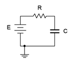
Figure 8.4.1 : A simple RC circuit.
The key to the analysis is to remember that capacitor voltage cannot change instantaneously. Assuming the capacitor is uncharged, the instant power is applied, the capacitor voltage must be zero. Therefore all of the source voltage drops across the resistor. This creates the initial current, and this current starts to charge the capacitor (the initial rate being equal to \(i/C\) as dictated by Equation 8.2.6). According to Kirchhoff's voltage law, as the capacitor voltage begins to increase, the resistor voltage must decrease because the sum of the two must equal the fixed source voltage. This means that the circulating current must also decrease. This, in turn, means that the rate of capacitor voltage increase begins to slow. As the capacitor voltage continues to increase, less voltage is available for the resistor, causing further reductions in current, and a further slowing of the rate of capacitor voltage change. Eventually, the capacitor voltage will be nearly equal to the source voltage. This will result in a very small potential across the resistor and an equally small current, slowing subsequent capacitor voltage increases to a near standstill. Theoretically, the capacitor voltage approaches the source voltage but never quite equals it. Similarly, the current drops to near zero, but never completely turns off. This is illustrated in Figure 8.4.2 .
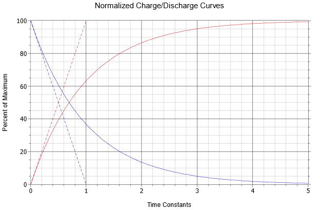
Figure 8.4.2 : Normalized charge and discharge curves.
The dashed red line represents the initial rate of change of capacitor voltage. This trajectory is what would be expected if an ideal current source drove the capacitor, as in Example 8.2.4. As noted previously, the rate of voltage change versus times is equal to \(i/C\), and therefore in this case, \(E/RC\). If the initial rate of change were to continue unabated, the source voltage, \(E\), would be reached in \(RC\) seconds. Consequently, RC is referred to as the charge time constant and is denoted by \(\tau \) (Greek letter tau). Thus,
\[\text{Time constant, } \tau = RC \label{8.10} \]
As noted, once the capacitor begins to charge, the current begins to decrease and the capacitor voltage curve begins to fall away from the initial trajectory. The solid red curve represents the capacitor voltage. Notice that after five time constants the capacitor is nearly fully charged and the circuit is considered to be in steady-state (i.e., the capacitor behaves as an open).
\[\text{Steady-state is reached in approximately five time constants.} \label{8.11} \]
This sort of recursively dependent operation is characteristic of exponential functions. The equation for the capacitor's voltage charging curve is:
\[V_C (t) = E\left(1 − \epsilon^{− \frac{t}{\tau}} \right) \label{8.12} \]
Where
\(V_C(t)\) is the capacitor voltage at time \(t\),
\(E\) is the source voltage,
\(t\) is the time of interest,
\(\tau\) is the time constant,
\(\varepsilon\) (also written \(e\)) is the base of natural logarithms, approximately 2.718.
The dashed blue line shows the initial slope of current change. The solid blue curve shows the circulating current (and by extension of Ohm's law, the resistor voltage). The equation for this curve, which follows the general shape \(\varepsilon^{ −t}\), is:
\[I (t)= \frac{E}{R} \epsilon^{ − \frac{t}{\tau}} \label{8.13} \]
and
\[V_R (t) = E \epsilon^{- \frac{t}{\tau}} \label{8.14} \]
Once power is removed or bypassed, the stored charge on the capacitor will dissipate through any associated resistor(s) creating a discharge current which will end with the capacitor voltage drained back to zero. During the discharge phase, both the capacitor's voltage and current will follow the solid blue curve; Equations \ref{8.13} and \ref{8.14} being appropriate. The discharge time constant may be different from the charge times constant, depending on the associated resistances.
A precise derivation of the exponential charge/discharge equations is given in Appendix C.
Given the circuit of Figure 8.4.3 , assume the switch is closed at time \(t = 0\). Determine the charging time constant, the amount of time after the switch is closed before the circuit reaches steady-state, and the capacitor voltage at \(t = 0\), \(t = 50\) milliseconds and \(t = 1\) second. Assume the capacitor is initially uncharged.
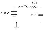
Figure 8.4.3 : Circuit for Example 8.4.1 .
First, the time constant:
\[\tau = RC \nonumber \]
\[\tau = 50 k \Omega 2 \mu F \nonumber \]
\[\tau = 100ms \nonumber \]
Steady-state will be reached in five time constants, or 500 milliseconds. Therefore we know that \(V_C(0) = 0\) volts and \(V_C(1) = 100\) volts. To find \(V_C(50 ms)\) we simply solve Equation \ref{8.12}.
\[V_C (t) = E \left(1 − \epsilon^{− \frac{t}{\tau}} \right) \nonumber \]
\[V_C (50 ms) = 100 V \left( 1 − \epsilon^{− \frac{50 ms}{100 ms}} \right) \nonumber \]
\[V_C (50 ms) \approx 39.35 V \nonumber \]
This value can also be determined graphically from Figure 8.4.2 . The time of 50 milliseconds represents one-half time constant. Find this value on the horizontal axis and then track straight up to the solid red curve that represents the charging capacitor voltage. The point of intersection is at approximately 40% of the maximum value on the vertical axis. The maximum value here is the source voltage of 100 volts. Therefore the capacitor will have reached approximately 40% of 100 volts, or just about 40 volts.
Computer Simulation
The circuit of Figure 8.4.3 is entered into a simulator, as shown in Figure 8.4.4 . In order to reflect the notion of a time-varying circuit with a switch, the 100 volt DC voltage source has been replaced with a rectangular pulse voltage source. This source starts at 0 volts and then immediately steps up to 100 volts. It stays at this level for 500 milliseconds before dropping back to 0 volts.
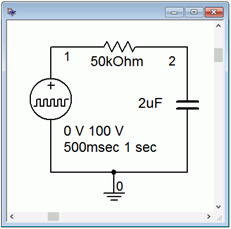
Figure 8.4.4 : Circuit of Figure 8.4.3 in a simulator.
A transient (i.e., time domain) simulation is run, plotting the capacitor voltage over time for the first 500 milliseconds. This is seen in Figure 8.4.5 . There are several items to note here. First, we see that the overall shape perfectly echoes the generic curve presented in Figure 8.4.2 . Second, we see that after the predicted five time constants, or 500 milliseconds, the capacitor voltage has plateaued, indicating steady-state. Third, at steady-state the capacitor voltage has virtually reached the maximum value set be the source, or 100 volts. Finally, at 50 milliseconds, we see that the capacitor voltage has reached roughly 40 volts, just as predicted.
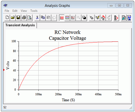
Figure 8.4.5 : Simulation results for the circuit of Figure 8.4.2 .
As mentioned previously, it is possible for a circuit to have different charge and discharge time constants. This could occur if a switch introduces or removes component(s) between the charge versus discharge phases. Further, because the capacitor is discharging, its current direction will be opposite to that of the charging current. KVL still must be satisfied, but because the capacitor is now behaving as a source, the magnitude of the discharge resistance's voltage must equal the capacitor voltage magnitude. Therefore, its curve will take the same shape (the solid blue curve of Figure 8.4.2 ). These issues will be illustrated in the following example.
For the circuit of Figure 8.4.6 , assume the capacitor is initially uncharged. At time \(t = 0\) the switch contacts position 1. The switch is thrown to position 2 at time \(t = 50\) milliseconds.
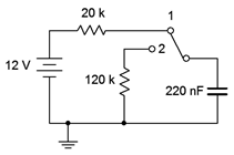
Figure 8.4.6 : Circuit for Example 8.4.2 .
Determine the charging time constant, the amount of time after the switch is closed before the circuit reaches steady-state, the maximum charging and discharging currents, and the capacitor voltage at \(t = 0\), \(t = 50\) milliseconds, \(t = 90\) milliseconds, and \(t = 1\) second.
We begin with the charge time constant:
\[\tau_{charge} = RC \nonumber \]
\[\tau_{charge} = 20 k \Omega 220 nF \nonumber \]
\[\tau_{charge} = 4.4 ms \nonumber \]
Steady-state will be reached in 5 times 4.4 milliseconds, or 22 milliseconds. The capacitor is initially uncharged, so \(V_C(0) = 0\) volts. As the capacitor will have reached steady-state in 22 milliseconds, \(V_C(50 ms) = 12\) volts. The maximum charging current will occur at \(t = 0\) when all of the 12 volt source drops across the 20 k\( \Omega \) resistor, or 600 \(\mu\)amps, flowing left to right.
At 50 milliseconds the switch is thrown to position 2. The 12 volt source and 20 k\( \Omega \) resistor are no longer engaged. At this point the capacitor has 12 volts across it, positive to negative, top to bottom. As the capacitor voltage cannot change instantaneously, the capacitor now acts as a voltage source and discharges through the 120 k\( \Omega \) resistor. Note that the discharge current is flowing counterclockwise, the opposite of the charging current. The discharge time constant is:
\[\tau_{discharge} = RC \nonumber \]
\[\tau_{discharge} = 120 k \Omega 220 nF \nonumber \]
\[\tau_{discharge} = 26.4 ms \nonumber \]
The capacitor will fully discharge down to 0 volts in 5 time constants, or some 132 milliseconds after the switch is thrown to position 2. Thus steady-state occurs at \(t = 182\) milliseconds. The maximum discharge current occurs the instant the switch is thrown to position 2 when all of the capacitor's 12 volts drops across the 120 k\( \Omega \) resistor, yielding 100 \(\mu\) amps, flowing top to bottom.
Clearly, at \(t = 90\) milliseconds the capacitor is in the discharge phase. The capacitor's voltage and current during the discharge phase follow the solid blue curve of Figure 8.4.2 . The elapsed time for discharge is 90 milliseconds minus 50 milliseconds, or 40 milliseconds net. We can use a slight variation on Equation \ref{8.14} to find the capacitor voltage at this time.
\[V_C (t) = E \epsilon^{− \frac{t}{\tau}} \nonumber \]
\[V_C (40 ms) = 12 V− \epsilon^{− \frac{40ms}{26.4 ms}} \nonumber \]
\[V_C (40 ms) \approx 2.637V \nonumber \]
The shape of the capacitor's voltage will appear somewhat like a rounded pulse, rising with a curve and then falling back to zero with a complementary curve (the red and then blue curves of Figure 8.4.2 ).
Basic single resistor-capacitor circuits prove to be fairly easy to solve given a little practice, but what if a more complex circuit is used? In this situation the section feeding the capacitor may be simplified using Thévenin's theorem to determine the effective source voltage and charging resistance. The circuit then reverts back to a simple RC network which may be solved directly.
If power is interrupted before the capacitor is fully charged, the equations presented previously may be used to determine the precise voltage(s) and current(s) reached. The capacitor will then behave as a voltage source and begin to discharge, its voltage curve following the blue plot line of Figure 8.4.2 , with its maximum voltage being what the capacitor charged to, not the associated driving voltage. The following example and simulations address these issues.
For this example we shall revisit the circuit of Example 8.3.1. The circuit is redrawn in Figure 8.4.7 for convenience. Assume the capacitor is initially uncharged.
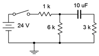
Figure 8.4.7 : Circuit for Example 8.4.3 .
Determine the charging time constant, the amount of time after the switch is closed before the circuit reaches steady-state, and the capacitor voltage at \(t = 0\), 100 milliseconds, and 200 milliseconds. At 200 milliseconds, the switch is opened. Determine how long it takes for the capacitor to fully discharge and the voltage across the 6 k\( \Omega \) resistor at \(t = 275\) milliseconds (i.e., 75 milliseconds after the switch is opened).
The first step is to determine the Thévenin equivalent driving the capacitor. If we remove the capacitor and determine the open circuit voltage at those points, we see that it is just a voltage divider between the 24 volt source, the 6 k\( \Omega \) resistor and the 1 k\( \Omega \) resistor (the 3 k\( \Omega \) resistor has no current through it and thus produces no voltage drop). This works out to 20.57 volts. The Thévenin resistance will be 3 k\( \Omega \) in series with 1 k\( \Omega \) \(||\) 6 k\( \Omega \), or roughly 3.857 k\( \Omega \). The equivalent charging circuit is drawn in Figure 8.4.8 .
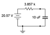
Figure 8.4.8 : Thévenin equivalent for the circuit of Figure 8.4.7 driving the capacitor.
We can now determine the charging time constant:
\[\tau_{charge} = RC \nonumber \]
\[\tau_{charge} = 3.857 k \Omega 10 \mu F \nonumber \]
\[\tau_{charge} = 38.57 ms \nonumber \]
Steady-state will be reached in 5 time constants, or 192.8 ms. Thus, we know that \(V_C(0) = 0\) volts and \(V_C(200 ms) = 20.57\) volts. For the capacitor voltage at 100 milliseconds, we simply use the charge equation.
\[V_C (t)= E \left(1−\epsilon^{− \frac{t}{\tau}} \right) \nonumber \]
\[V_C (100ms) = 20.57 V \left(1− \epsilon^{− \frac{100 ms}{38.57ms}} \right) \nonumber \]
\[V_C (100ms) \approx 19.03 V \nonumber \]
For the discharge phase, we need to determine the time constant. With the voltage source removed, the capacitor will discharge through the now series combination of the 3 k\( \Omega \) resistor and 6 k\( \Omega \) resistor.
\[\tau_{discharge} = RC \nonumber \]
\[\tau_{discharge} = 9k \Omega 10 \mu F \nonumber \]
\[\tau_{discharge} = 90 ms \nonumber \]
Steady-state will be reached 450 milliseconds later at \(t = 650\) milliseconds. To find \(V_{6k}\) at \(t = 275\) milliseconds, we can find the voltage across the capacitor and then perform a voltage divider between the 6 k\(\Omega\) and 3 k\(\Omega\) resistors. Remembering that \(t = 275\) milliseconds is 75 milliseconds into the discharge phase, we have:
\[V_C (t) = E \epsilon^{− \frac{t}{\tau}} \nonumber \]
\[V_C (75 ms) = 20.57V \left( 1− \epsilon^{− \frac{75ms}{90ms}} \right) \nonumber \]
\[V_C (75 ms) \approx 8.94 V \nonumber \]
Finally, this voltage splits between the 6 k\( \Omega \) and 3 k\( \Omega \) resistors. Using the voltage divider rule, we find:
\[V_{6k} = V_C \frac{R_x}{R_x+R_y} \nonumber \]
\[V_{6k} = 8.94 V \frac{6 k \Omega }{6 k \Omega +3k \Omega } \nonumber \]
\[V_{6k} = 5.96 V \nonumber \]
Computer Simulation
In order to verify the analysis of Example 8.4.3 , the circuit of Figure 8.4.7 is entered into a simulator, as shown in Figure 8.4.9 . In place of a DC source, a pulse generator is used to mimic the on-off nature of the switch. This starts starts at zero volts and then immediately jumps up to 24 volts. It stays at this level for 200 milliseconds before returning back to zero. This is sufficient time to check whether or not the capacitor voltage has reached steady-state (predicted to take 192.8 milliseconds).
Figure 8.4.9 : Circuit of Figure 8.4.7 in a simulator.
A transient analysis is run on this circuit, plotting the capacitor voltage (i.e., the difference between the node 2 and node 3 voltages). The result is shown in Figure 8.4.10 . This plot confirms nicely the charge phase of the capacitor. After approximately 200 milliseconds, the voltage has leveled out at just over 20 volts, precisely as predicted.
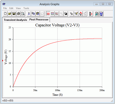
Figure 8.4.10 : Simulation results for the charge phase of the circuit of Figure 8.4.7 .
What about the discharge phase? In order to investigate that portion, the simulation circuit is modified. The pulse voltage source is disconnected from the remainder of the circuit, just as it would be if the switch in Figure 8.4.7 had been opened again. Also, the capacitor is modified to have an initial voltage of 20.57 volts, the precise value at had reached after it attained steady-state. A second transient analysis is run, again plotting the capacitor voltage. The results of this simulation are shown in Figure 8.4.11 . It is worth noting that the time axis is relative to the switch being opened, not the original timing. That is, the horizontal origin of 0 milliseconds corresponds to \(t = 200\) milliseconds.
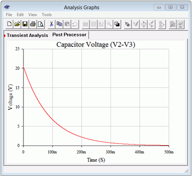
Figure 8.4.11 : Simulation results for the discharge phase of the circuit of Figure 8.4.7 .
Note that the time required to reach the new steady-state value of zero volts has stretched out to some 450 milliseconds after the switch is opened, precisely as predicted.
At this point, a fair question to ask is, “Couldn't we leave the pulse source in place in order to investigate the discharge phase?” Although the pulse source does go back down to zero volts at \(t = 200\) milliseconds, that's not the same as opening the switch back in Figure 8.4.7 . If the source is still connected but producing zero volts, it becomes part of the Thévenin equivalent. As such, the 1 k\( \Omega \) resistor is back in the circuit, producing a discharge time constant identical to the charge time constant.
To prove the point, the simulation is run again. The pulse remains at 24 volts for 200 milliseconds and then jumps down to zero, as before. The simulation time is extended out to 400 milliseconds total, enough to see both the charge and discharge phases. Further, instead of just plotting the capacitor voltage; the voltages of the source (blue trace, node 1), the 6 k\( \Omega \) resistor (green trace, node 2) and the 3 k\( \Omega \) resistor (red trace, node 5) are plotted. The results are shown in Figure 8.4.12 .
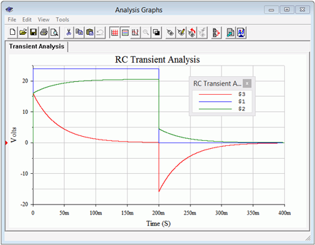
Figure 8.4.12 : Simulation results using pulse voltage source for discharge phase.
The first item to note is that steady-state appears to be reached in just under 200 milliseconds for both the charge and discharge phases, as expected. Second, note that the node 2 voltage (green) minus the node 3 voltage (red) starts at zero and winds up at a little over 20 volts at 200 milliseconds. This is, of course, the capacitor voltage, but what is interesting here is that this plot shows how the voltage across the 3 k\( \Omega \) resistor shrinks as the capacitor voltage grows, the sum equaling the node 2 voltage. This makes perfect sense because, as the capacitor voltage increases, the current through it must be decreasing, and as this same current is flowing through the 3 k\( \Omega \) resistor, the resistor's voltage must also be decreasing due to Ohm's law.
The other interesting part of this plot is what happens at 200 milliseconds when the source goes back to zero. Note that the node 3 voltage immediately jumps to a negative value. This is because the voltage across the capacitor cannot change instantaneously. It must still have 20.57 volts across it the instant the source goes back to zero. In this situation, because the source is essentially a short, the capacitor winds up in series with the 3 k\( \Omega \) resistor and the parallel combination of the 1 k\( \Omega \) and 6 k\( \Omega \) resistors, or about 857 \( \Omega \). Calculating the voltage divider between the 3 k\( \Omega \) and 857 \( \Omega \) resistors with 20.57 volt source shows the 3 k\( \Omega \) resistor receiving approximately 16 volts. Further, the discharge current will be flowing out of the capacitor in a counterclockwise direction, meaning it flows from ground up through the 3 k\( \Omega \) resistor. Thus, we expect node 3 to be at approximately −16 volts, which is precisely what the plot indicates. How cool is that?
What if we didn't wait for steady-state? How would these plots change? Essentially, the trajectories of the curves would not change. After all, how would the circuit “know” that the switch would open early or the pulse would flip prematurely?
What happens is that the curves are followed to the point in time where the circuit is interrupted. From there, the next phase occurs with the present voltages as the starting points. To test this, the simulation is run yet again, but this time the source pulse width is shortened to just 50 milliseconds, well short of steady-state. The results of the simulation are shown in Figure 8.4.13 .
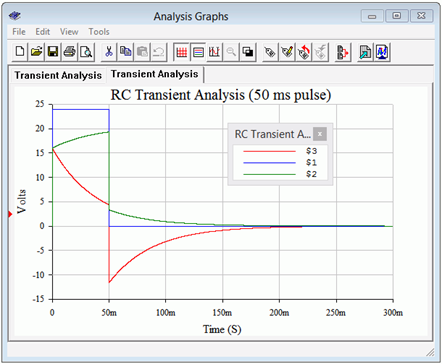
Figure 8.4.13 : Simulation results for interrupted discharge phase using pulse voltage source.
Comparing the plot of Figure 8.4.13 to that of Figure 8.4.12 shows that the two are identical up to 50 milliseconds. At that point, the input pulse returns to zero and the capacitor begins to discharge. The shapes and timings of the node 2 and node 3 voltages are the same as they were in Figure 8.4.12 , however, the amplitudes are reduced. This is because the capacitor did not have time to reach the steady-state voltage of 20.57 volts. In fact, it only reaches about 14.94 volts using Equation \ref{8.12}. Applying the voltage divider on this potential as before shows that the 3 k\( \Omega \) resistor should jump to approximately −11.6 volts, which is confirmed by the simulation.