1.5: The Double Slit Experiment

Last updated
Save as PDF

Page ID: 49368

Marc Baldo
Massachusetts Institute of Technology via MIT OpenCourseWare

\( \newcommand{\vecs}[1]{\overset { \scriptstyle \rightharpoonup} {\mathbf{#1}} } \) \( \newcommand{\vecd}[1]{\overset{-\!-\!\rightharpoonup}{\vphantom{a}\smash {#1}}} \)\(\newcommand{\id}{\mathrm{id}}\) \( \newcommand{\Span}{\mathrm{span}}\) \( \newcommand{\kernel}{\mathrm{null}\,}\) \( \newcommand{\range}{\mathrm{range}\,}\) \( \newcommand{\RealPart}{\mathrm{Re}}\) \( \newcommand{\ImaginaryPart}{\mathrm{Im}}\) \( \newcommand{\Argument}{\mathrm{Arg}}\) \( \newcommand{\norm}[1]{\| #1 \|}\) \( \newcommand{\inner}[2]{\langle #1, #2 \rangle}\) \( \newcommand{\Span}{\mathrm{span}}\) \(\newcommand{\id}{\mathrm{id}}\) \( \newcommand{\Span}{\mathrm{span}}\) \( \newcommand{\kernel}{\mathrm{null}\,}\) \( \newcommand{\range}{\mathrm{range}\,}\) \( \newcommand{\RealPart}{\mathrm{Re}}\) \( \newcommand{\ImaginaryPart}{\mathrm{Im}}\) \( \newcommand{\Argument}{\mathrm{Arg}}\) \( \newcommand{\norm}[1]{\| #1 \|}\) \( \newcommand{\inner}[2]{\langle #1, #2 \rangle}\) \( \newcommand{\Span}{\mathrm{span}}\)\(\newcommand{\AA}{\unicode[.8,0]{x212B}}\)

We now have the tools to model the double slit experiment described above. Far from the double slit, the electrons emanating from each slit look like plane waves; see Figure \(\PageIndex{1}\), where \(s\) is the separation between the slits and \(L\) is the distance to the viewing screen.

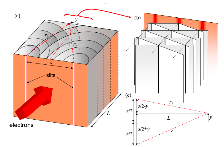
Screenshot 2021-04-14 at 08.53.29.png — Figure \(\PageIndex{1}\): Far from the double slit, the electrons from each slit can be described by plane waves. Where the planes of constant phase collide, a bright line corresponding to a high intensity of electrons is observed.

At the viewing screen we have

\[ \psi(x=L,t) = A\text{ exp}[i(k_{0}r_{1}-\omega_{0}t)]+A\text{ exp}[i(k_{0}r_{2}-\omega_{0}t)] \nonumber \]

The intensity at the screen is

\[ \begin{align*} |\psi|^{2} &= \{ A \text{ exp}[-i\omega_{0}t](\text{exp}[ik_{0}r_{1}]+(\text{exp}[ik_{0}r_{1}])\}\{A \text{ exp}[-i\omega_{0}t](\text{exp}[ik_{0}r_{1}]+(\text{exp}[ik_{0}r_{1}])^{*} \\[4pt] &= |A|^{2} + |A|^{2}\text{ exp}[i(k_{0}r_{2}-k_{0}r_{1})]+|A|^{2}\text{ exp}[i(k_{0}r_{1}-k_{0}r_{2})]+|A|^{2} \\[4pt] &=2|A|^{2} (1+cos(k(r_{2}-r_{1}))) \end{align*} \nonumber \]

where \(A\) is a constant determined by the intensity of the electron wave. Now from Figure \(\PageIndex{1}\):

\[ r^{2}_{1}= L^{2}+(s/2 -y)^{2} \nonumber \]

\( r^{2}_{1}= L^{2}+(s/2 +y)^{2} \)

Now, if \(y \ll s/2\) we can neglect the \(y^{2}\) term:

\[ r^{2}_{1}= L^{2}+(s/2)^{2}-sy \nonumber \]

\( r^{2}_{1}= L^{2}+(s/2)^{2}+sy \)

Then,

\[ r_{1} \approx \sqrt{L^{2}+(s/2)^{2}}(1-\dfrac{1}{2}\dfrac{sy}{L^{2}+(s/2)^{2}}) \nonumber \]

\( r_{1} \approx \sqrt{L^{2}+(s/2)^{2}}(1+\dfrac{1}{2}\dfrac{sy}{L^{2}+(s/2)^{2}}) \)

Next, if \(L \gg s/2\)

\[ r_{1} \approx L-\dfrac{1}{2}\dfrac{sy}{L} \nonumber \]

\( r_{1} \approx L+\dfrac{1}{2}\dfrac{sy}{L} \)

Thus, \(r_{2}-r_{1} = \dfrac{sy}{L}\), and

\[ |\psi|^{2} = 2|A|^{2} (1+cos(ks\dfrac{y}{L})) \nonumber \]

At the screen, constructive interference between the plane waves from each slit yields a regular array of bright lines, corresponding to a high intensity of electrons. In between each pair of bright lines, is a dark band where the plane waves interfere destructively, i.e. the waves are \(\pi\) radians out of phase with one another.

\[ \dfrac{2\pi}{\lambda}s\dfrac{y}{L}=2\pi \nonumber \]

Rearranging,

\[ y=\dfrac{L\lambda}{s} \nonumber \]