1.25: The Square Well

Last updated
Save as PDF

Page ID: 50126

Marc Baldo
Massachusetts Institute of Technology via MIT OpenCourseWare

\( \newcommand{\vecs}[1]{\overset { \scriptstyle \rightharpoonup} {\mathbf{#1}} } \) \( \newcommand{\vecd}[1]{\overset{-\!-\!\rightharpoonup}{\vphantom{a}\smash {#1}}} \)\(\newcommand{\id}{\mathrm{id}}\) \( \newcommand{\Span}{\mathrm{span}}\) \( \newcommand{\kernel}{\mathrm{null}\,}\) \( \newcommand{\range}{\mathrm{range}\,}\) \( \newcommand{\RealPart}{\mathrm{Re}}\) \( \newcommand{\ImaginaryPart}{\mathrm{Im}}\) \( \newcommand{\Argument}{\mathrm{Arg}}\) \( \newcommand{\norm}[1]{\| #1 \|}\) \( \newcommand{\inner}[2]{\langle #1, #2 \rangle}\) \( \newcommand{\Span}{\mathrm{span}}\) \(\newcommand{\id}{\mathrm{id}}\) \( \newcommand{\Span}{\mathrm{span}}\) \( \newcommand{\kernel}{\mathrm{null}\,}\) \( \newcommand{\range}{\mathrm{range}\,}\) \( \newcommand{\RealPart}{\mathrm{Re}}\) \( \newcommand{\ImaginaryPart}{\mathrm{Im}}\) \( \newcommand{\Argument}{\mathrm{Arg}}\) \( \newcommand{\norm}[1]{\| #1 \|}\) \( \newcommand{\inner}[2]{\langle #1, #2 \rangle}\) \( \newcommand{\Span}{\mathrm{span}}\)\(\newcommand{\AA}{\unicode[.8,0]{x212B}}\)

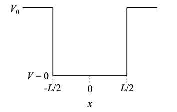
Next we consider a single electron within a square potential well as shown in Figure 1.25.1. As mentioned in the discussion of the photoelectric effect, electrons within solids are bound by attractive nuclear forces.

By modeling the binding energy within a solid as a square well, we entirely ignore fine scale structure within the solid. Hence the square well, or particle in a box, as it is often known, is one of the crudest approximations for an electron within a solid. The simplicity of the square well approximation, however, makes it one of the most useful problems in all of quantum mechanics.

Screenshot 2021-04-15 at 10.50.18.png — Figure \(\PageIndex{1}\): The square well. Within the solid the potential is defined to be zero. In free space, outside the solid, the repulsive potential is \(V_{0}\).

Since the potential changes abruptly, we treat each region of constant potential separately. Subsequently, we must connect up the solutions in the different regions. Tackling the problem this way is known as a piecewise solution.

Now, the Schrödinger Equation is a statement of the conservation of energy

\[ \text{total energy (E)} = \text{kinetic energy (KE)}+\text{Potential energy (V)} \nonumber \]

In classical mechanics, one can never have a negative kinetic energy. Thus, classical mechanics requires that E > V. This is known as the classically allowed region.

But in our quantum analysis, we will find solutions for E < V. This is known as the classically forbidden regime.

The classically allowed region

Rearranging Equation (1.23.5) gives the second order differential equation:

\[ \frac{d^{2}\psi}{dx^{2}} = -\frac{2m(E-V)}{\hbar^{2}}\psi \nonumber \]

In this region, E > V, solutions are of the form

\[ \psi(x)=Ae^{ikx}+Be^{-ikx} \nonumber \]

\[ \psi(x)=A\ sin(kx)+B\ cos(kx) \nonumber \]

where

\[ k =\sqrt{\frac{2m(E-V)}{\hbar^{2}}} \nonumber \]

In the classically allowed region we have oscillating solutions.

The classically forbidden region

In this region, E < V, and solutions are of the form

\[ \psi(x)=Ae^{\alpha x} +Be^{-\alpha x} \nonumber \]

i.e. they are either growing or decaying exponentials where

\[ \alpha = \sqrt{\frac{2m(V-E)}{\hbar^{2}}} \nonumber \]