2.4: Metals and Insulators

Last updated
Save as PDF

Page ID: 50019

Marc Baldo
Massachusetts Institute of Technology via MIT OpenCourseWare

\( \newcommand{\vecs}[1]{\overset { \scriptstyle \rightharpoonup} {\mathbf{#1}} } \) \( \newcommand{\vecd}[1]{\overset{-\!-\!\rightharpoonup}{\vphantom{a}\smash {#1}}} \)\(\newcommand{\id}{\mathrm{id}}\) \( \newcommand{\Span}{\mathrm{span}}\) \( \newcommand{\kernel}{\mathrm{null}\,}\) \( \newcommand{\range}{\mathrm{range}\,}\) \( \newcommand{\RealPart}{\mathrm{Re}}\) \( \newcommand{\ImaginaryPart}{\mathrm{Im}}\) \( \newcommand{\Argument}{\mathrm{Arg}}\) \( \newcommand{\norm}[1]{\| #1 \|}\) \( \newcommand{\inner}[2]{\langle #1, #2 \rangle}\) \( \newcommand{\Span}{\mathrm{span}}\) \(\newcommand{\id}{\mathrm{id}}\) \( \newcommand{\Span}{\mathrm{span}}\) \( \newcommand{\kernel}{\mathrm{null}\,}\) \( \newcommand{\range}{\mathrm{range}\,}\) \( \newcommand{\RealPart}{\mathrm{Re}}\) \( \newcommand{\ImaginaryPart}{\mathrm{Im}}\) \( \newcommand{\Argument}{\mathrm{Arg}}\) \( \newcommand{\norm}[1]{\| #1 \|}\) \( \newcommand{\inner}[2]{\langle #1, #2 \rangle}\) \( \newcommand{\Span}{\mathrm{span}}\)\(\newcommand{\AA}{\unicode[.8,0]{x212B}}\)

Metals are good conductors; a small difference between \(F^{+}\) and \(F^{-}\) yields a large difference between the number of electrons in \(+k_{z}\) and \(-k_{z}\) states. This is possible if the bands are partially filled at equilibrium.

If there are no electrons between \(F^{+}\) and \(F^{-}\), then the material is an insulator and cannot conduct charge. This occurs if the bands are completely empty or completely full at equilibrium. We have not yet encountered a band that can be completely filled. These will come later in the class.

Thus, to calculate the current in a material, we must determine the number of electrons in states that lie between the quasi Fermi levels. It is often convenient to approximate Equation 2.2.2 when calculating the number of electrons in a material. There are two limiting cases:

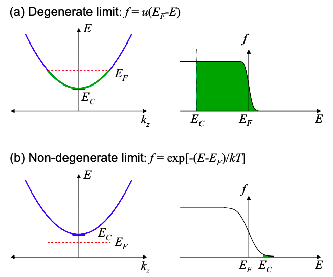
degenerate limit: \(E_{F}-E_{C} \ggkT\).

As shown in Figure 2.4.1(a), here the bottom of the band, \(E_{C}\), is much less than the Fermi energy, \(E_{F}\), and the distribution function is modeled by a unit step:

\[ f(E) = u(E_{F}-E) \nonumber \]

non-degenerate limit: \(E_{C}-E_{F} \ggkT\).

As shown in Figure 2.4.1(b), here \(E_{C} \geq E_{F}\) and the distribution function reduces to the Boltzmann distribution:

\[ f(E) = \text{exp}[-(E-E_{f})/kT] \nonumber \]

Screenshot 2021-04-15 at 21.23.03.png — Figure \(\PageIndex{1}\): Two limiting cases when calculating the number of electrons in a material. (a) If \(E_{F}\) is within a band, then thermal blurring of the electron distribution is not significant, and we can simply integrate up to \(E_{F}\). This is the so-called degenerate case. (b) On the other hand, if the filled states are due solely to thermal excitation above \(E_{F}\), the filling fraction falls off exponentially. This is the non-degenerate limit.