4.1: Two Terminal Quantum Wire Devices

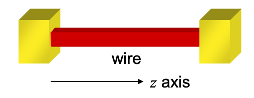
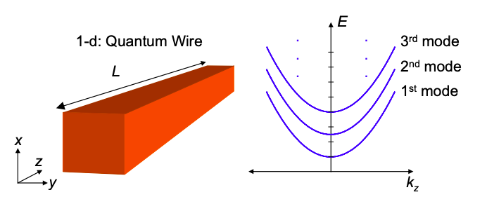
Let's consider a quantum wire between two contacts. As we saw in Part 2, a quantum wire is a one-dimensional conductor. Here, we will assume that the wire has the same geometry as studied in Part 2: a rectangular cross section with area Lx.Ly. Electrons are confined by an infinite potential outside the wire, and can only flow along its length; arbitrarily chosen as the z-axis in Figure 4.1.1.

Figure \(\PageIndex{1}\): A quantum wire between two contacts.

Under these assumptions, if we model the electrons by plane waves in the z direction we get

\[ E=\frac{\pi^{2}\hbar^{2}}{2m} \left( \frac{n^{2}_{x}}{L^{2}_{x}} +\frac{n^{2}_{y}}{L^{2}_{y}} \right) + \frac{\hbar^{2}k_{z}^{2}}{2m}, \ \ \ n_{x},n_{y} = 1,2,… \nonumber \]

Figure \(\PageIndex{2}\): Plane waves in a quantum wire have parabolic energy bands.

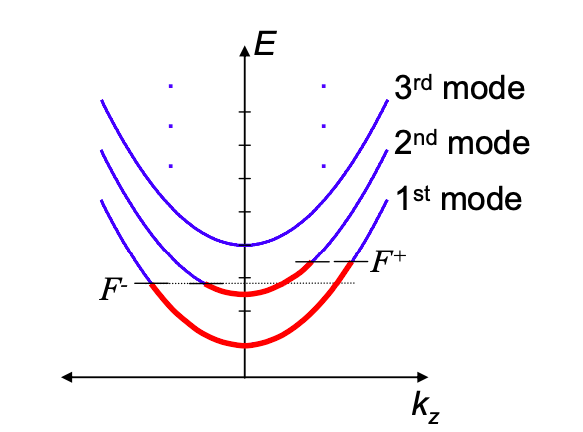
Recall that for current to flow there must be difference in the number of electrons in \(+k_{z}\) and \(-k_{z}\) states. As in Part 2, we define two quasi Fermi levels: \(F^{+}\) for states with \(k_{z}>0\), \(F^{-}\) for states with \(k_{z}<0\). Thus, current flows when electrons traveling in the +z direction are in equilibrium with each other, but not with electrons traveling in the –z direction. For example, in Figure 4.1.3, current is carried by the uncompensated electrons in the \(+k_{z}\) states.

Figure \(\PageIndex{3}\): Current flows when the quasi Fermi levels differ for +k_{z} and -k_{z}. states.