4.9: Ohm’s law

What happens when we increase the size of a conductor? Eventually, we should obtain Ohm's law as the quantum phenomena transform into the familiar model of classical conduction:

\[ V=IR \nonumber \]

But a linear relationship between V and I is not particularly profound. Almost any system can be linearized over a sufficiently narrow range of voltage or current. It is more significant to evaluate the resistance, R, in terms of macroscopic quantities such as crosssectional area, A, and length, L.

You might recall that resistance is classically defined as:

\[ R = \frac{\rho L}{A} . \nonumber \]

where \(\rho\), the resistivity, is some material dependent quantity, usually determined by a measurement. Let's see where this expression comes from – it will help illustrate differences between quantum and classical models of charge conduction.

At zero temperature, transmission formalism gives

\[ G = \frac{2q^{2}}{h} M \Im \nonumber \]

where M is the number of modes, and \(\Im\) is the net transmission coefficient. Rearranging this in terms of a resistance, we have

\[ R = \frac{h}{2q^{2}} \frac{1}{M \Im} \nonumber \]

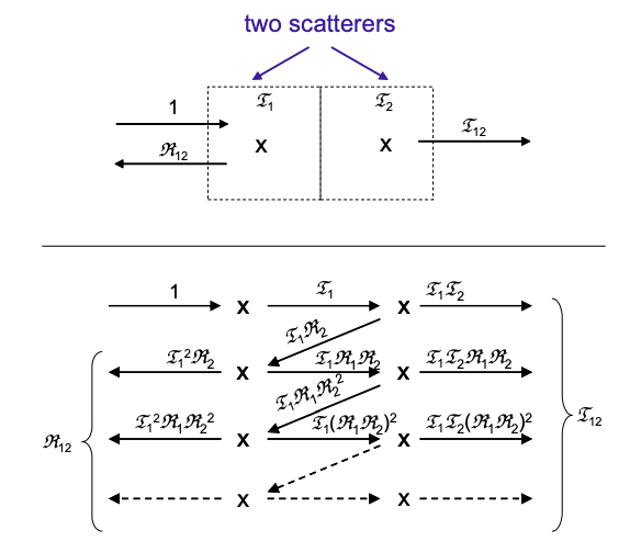
To determine the net transmission coefficient, let's break the conductor into a series of N elements labeled \(i = 1… N\), each containing a scattering site with transmission \(\Im_{i}\); see Figure 4.9.1.

For many scatterers there will be many reflections to consider. If the scattering mechanism preserves the phase information of the electrons, then multiple reflections can yield interference effects. Such scattering is said to be coherent. Here, we will consider only incoherent scattering that randomizes the electron phase.

Let's begin with just two incoherent scatterers in series. The transmission for two incoherent scatterers in series is:

\[ \Im_{12} = \Im_{1}\Im_{2}+ \Im_{1}\Im_{2}\Re_{1}\Re_{2}+\Im_{1}\Im_{2}(\Re_{1}\Re_{2})^{2} + … \nonumber \]

where \(\Re_{i}\) is the reflection from the ith scatterer, and \(\Im_{i}=(1-\Re_{i})\).

Figure \(\PageIndex{1}\): Two scatterers generate an infinite number of reflections, but we can sum the geometric series. Adapted from S. Datta, "Electronic Transport in Mesoscopic Systems" Cambridge (1995).

This geometric series simplifies to

\[ \Im_{12}= \frac{\Im_{1}\Im_{2}}{1-\Re_{1}\Re_{2}} , \nonumber \]

We can rearrange Eq. (4.9.6) to show

\[ \frac{\Re_{12}}{\Im_{12}} = \frac{\Re_{1}}{\Im_{1}} + \frac{\Re_{2}}{\Im_{2}} \nonumber \]

Thus, for N identical scatterers:

\[ \frac{\Re}{\Im} = N\frac{\Re_{i}}{\Im_{i}} \nonumber \]

Solving for the net transmission and using \(\Im=(1-\Re)\)

\[ \Im=\frac{\Im_{i}}{N(1-\Im_{i})+\Im_{i}} \nonumber \]

If we have \(\lambda\) scatterers per unit length, then

\[ \tau=\frac{\tau_{i}}{\lambda L(1-\Im_{i})+\Im_{i}}=\frac{L_{0}}{L+L_{0}} \nonumber \]

Thus, Equation (4.9.4) becomes

\[ R = \frac{h}{2q^{2}} \frac{1}{M}\left(1+\frac{L}{L_{0}}\right) \nonumber \]

where \(L_{0} = \Im/\lambda (1-\Im)\) is a characteristic length. The length dependence of resistance is clear from Equation (4.9.11). The dependence on cross sectional area is due to the number of current-carrying modes in the conductor

\[ M \approx \frac{k_{F}^{2}}{4\pi}A , \nonumber \]

where \(k_{F}\) is the Fermi wavevector.

Thus, we find that resistance can be broken into two components, a resistance due to the contacts, and a resistance that scales with the length of the conductor.

\[ R=R_{C}+R_{B}=\frac{\rho L_{0}}{A}+\frac{\rho L}{A} \nonumber \]

The contact resistance is the quantum effect that is familiar to us from Landauer theory. But in large conductors, the contact resistance is overwhelmed and we get the familiar classical expression for resistance.

\(^{†}\) This section is adapted from S. Datta, "Electronic Transport in Mesoscopic Systems" Cambridge (1995).