
1.11: Diffusion
- Page ID
- 88622

\( \newcommand{\vecs}[1]{\overset { \scriptstyle \rightharpoonup} {\mathbf{#1}} } \)
\( \newcommand{\vecd}[1]{\overset{-\!-\!\rightharpoonup}{\vphantom{a}\smash {#1}}} \)
\( \newcommand{\dsum}{\displaystyle\sum\limits} \)
\( \newcommand{\dint}{\displaystyle\int\limits} \)
\( \newcommand{\dlim}{\displaystyle\lim\limits} \)
\( \newcommand{\id}{\mathrm{id}}\) \( \newcommand{\Span}{\mathrm{span}}\)
( \newcommand{\kernel}{\mathrm{null}\,}\) \( \newcommand{\range}{\mathrm{range}\,}\)
\( \newcommand{\RealPart}{\mathrm{Re}}\) \( \newcommand{\ImaginaryPart}{\mathrm{Im}}\)
\( \newcommand{\Argument}{\mathrm{Arg}}\) \( \newcommand{\norm}[1]{\| #1 \|}\)
\( \newcommand{\inner}[2]{\langle #1, #2 \rangle}\)
\( \newcommand{\Span}{\mathrm{span}}\)
\( \newcommand{\id}{\mathrm{id}}\)
\( \newcommand{\Span}{\mathrm{span}}\)
\( \newcommand{\kernel}{\mathrm{null}\,}\)
\( \newcommand{\range}{\mathrm{range}\,}\)
\( \newcommand{\RealPart}{\mathrm{Re}}\)
\( \newcommand{\ImaginaryPart}{\mathrm{Im}}\)
\( \newcommand{\Argument}{\mathrm{Arg}}\)
\( \newcommand{\norm}[1]{\| #1 \|}\)
\( \newcommand{\inner}[2]{\langle #1, #2 \rangle}\)
\( \newcommand{\Span}{\mathrm{span}}\) \( \newcommand{\AA}{\unicode[.8,0]{x212B}}\)
\( \newcommand{\vectorA}[1]{\vec{#1}} % arrow\)
\( \newcommand{\vectorAt}[1]{\vec{\text{#1}}} % arrow\)
\( \newcommand{\vectorB}[1]{\overset { \scriptstyle \rightharpoonup} {\mathbf{#1}} } \)
\( \newcommand{\vectorC}[1]{\textbf{#1}} \)
\( \newcommand{\vectorD}[1]{\overrightarrow{#1}} \)
\( \newcommand{\vectorDt}[1]{\overrightarrow{\text{#1}}} \)
\( \newcommand{\vectE}[1]{\overset{-\!-\!\rightharpoonup}{\vphantom{a}\smash{\mathbf {#1}}}} \)
\( \newcommand{\vecs}[1]{\overset { \scriptstyle \rightharpoonup} {\mathbf{#1}} } \)
\(\newcommand{\longvect}{\overrightarrow}\)
\( \newcommand{\vecd}[1]{\overset{-\!-\!\rightharpoonup}{\vphantom{a}\smash {#1}}} \)
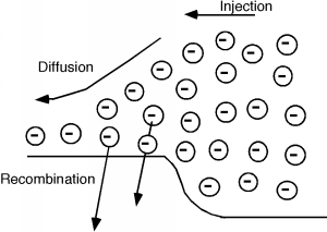
\(\newcommand{\avec}{\mathbf a}\) \(\newcommand{\bvec}{\mathbf b}\) \(\newcommand{\cvec}{\mathbf c}\) \(\newcommand{\dvec}{\mathbf d}\) \(\newcommand{\dtil}{\widetilde{\mathbf d}}\) \(\newcommand{\evec}{\mathbf e}\) \(\newcommand{\fvec}{\mathbf f}\) \(\newcommand{\nvec}{\mathbf n}\) \(\newcommand{\pvec}{\mathbf p}\) \(\newcommand{\qvec}{\mathbf q}\) \(\newcommand{\svec}{\mathbf s}\) \(\newcommand{\tvec}{\mathbf t}\) \(\newcommand{\uvec}{\mathbf u}\) \(\newcommand{\vvec}{\mathbf v}\) \(\newcommand{\wvec}{\mathbf w}\) \(\newcommand{\xvec}{\mathbf x}\) \(\newcommand{\yvec}{\mathbf y}\) \(\newcommand{\zvec}{\mathbf z}\) \(\newcommand{\rvec}{\mathbf r}\) \(\newcommand{\mvec}{\mathbf m}\) \(\newcommand{\zerovec}{\mathbf 0}\) \(\newcommand{\onevec}{\mathbf 1}\) \(\newcommand{\real}{\mathbb R}\) \(\newcommand{\twovec}[2]{\left[\begin{array}{r}#1 \\ #2 \end{array}\right]}\) \(\newcommand{\ctwovec}[2]{\left[\begin{array}{c}#1 \\ #2 \end{array}\right]}\) \(\newcommand{\threevec}[3]{\left[\begin{array}{r}#1 \\ #2 \\ #3 \end{array}\right]}\) \(\newcommand{\cthreevec}[3]{\left[\begin{array}{c}#1 \\ #2 \\ #3 \end{array}\right]}\) \(\newcommand{\fourvec}[4]{\left[\begin{array}{r}#1 \\ #2 \\ #3 \\ #4 \end{array}\right]}\) \(\newcommand{\cfourvec}[4]{\left[\begin{array}{c}#1 \\ #2 \\ #3 \\ #4 \end{array}\right]}\) \(\newcommand{\fivevec}[5]{\left[\begin{array}{r}#1 \\ #2 \\ #3 \\ #4 \\ #5 \\ \end{array}\right]}\) \(\newcommand{\cfivevec}[5]{\left[\begin{array}{c}#1 \\ #2 \\ #3 \\ #4 \\ #5 \\ \end{array}\right]}\) \(\newcommand{\mattwo}[4]{\left[\begin{array}{rr}#1 \amp #2 \\ #3 \amp #4 \\ \end{array}\right]}\) \(\newcommand{\laspan}[1]{\text{Span}\{#1\}}\) \(\newcommand{\bcal}{\cal B}\) \(\newcommand{\ccal}{\cal C}\) \(\newcommand{\scal}{\cal S}\) \(\newcommand{\wcal}{\cal W}\) \(\newcommand{\ecal}{\cal E}\) \(\newcommand{\coords}[2]{\left\{#1\right\}_{#2}}\) \(\newcommand{\gray}[1]{\color{gray}{#1}}\) \(\newcommand{\lgray}[1]{\color{lightgray}{#1}}\) \(\newcommand{\rank}{\operatorname{rank}}\) \(\newcommand{\row}{\text{Row}}\) \(\newcommand{\col}{\text{Col}}\) \(\renewcommand{\row}{\text{Row}}\) \(\newcommand{\nul}{\text{Nul}}\) \(\newcommand{\var}{\text{Var}}\) \(\newcommand{\corr}{\text{corr}}\) \(\newcommand{\len}[1]{\left|#1\right|}\) \(\newcommand{\bbar}{\overline{\bvec}}\) \(\newcommand{\bhat}{\widehat{\bvec}}\) \(\newcommand{\bperp}{\bvec^\perp}\) \(\newcommand{\xhat}{\widehat{\xvec}}\) \(\newcommand{\vhat}{\widehat{\vvec}}\) \(\newcommand{\uhat}{\widehat{\uvec}}\) \(\newcommand{\what}{\widehat{\wvec}}\) \(\newcommand{\Sighat}{\widehat{\Sigma}}\) \(\newcommand{\lt}{<}\) \(\newcommand{\gt}{>}\) \(\newcommand{\amp}{&}\) \(\definecolor{fillinmathshade}{gray}{0.9}\)Let us turn our attention to what happens to the electrons and holes, once they have been injected across a forward-biased junction. We will concentrate just on the electrons which are injected into the p-side of the junction, but keep in mind that similar things are also happening to the holes which enter the n-side.
As we saw a while back, when electrons are injected across a junction, they move away from the junction region by a diffusion process, while at the same time, some of them are disappearing because they are minority carriers (electrons in basically p-type material) and so there are lots of holes around for them to recombine with. This is all shown schematically in Figure \(\PageIndex{1}\).
Diffusion Process Quantified
It is actually fairly easy to quantify this, and come up with an expression for the electron distribution within the p-region. First we have to look a little bit at the diffusion process, however. Imagine that we have a series of bins, each with a different number of electrons in them. In a given time, we could imagine that all of the electrons would flow out of their bins into the neighboring ones. Since there is no reason to expect the electrons to favor one side over the other, we will assume that exactly half leave by each side. This is all shown in Figure \(\PageIndex{2}\). We will keep things simple and only look at three bins. Imagine I have 4, 6, and 8 electrons respectively in each of the bins. After the required "emptying time," we will have a net flux of exactly one electron across each boundary as shown.
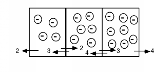 Figure \(\PageIndex{2}\): First example of a diffusion problem
Now let's raise the number of electrons to 8, 12 and 16 respectively (the electrons may overlap some now in the picture.) We find that the net flux across each boundary is now 2 electrons per emptying time, rather than one.
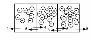
Note that the gradient (slope) of the concentration in the boxes has also doubled from one per box to two per box. This leads us to a rather obvious statement that the flux of carriers is proportional to the gradient of their density. This is stated formally in what is known as Fick's First Law of Diffusion: \[\text{Flux} = \left(-D_{e}\right) \frac{\text{d} n(x)}{\text{d} x} \nonumber \]
where \(D_{e}\) is simply a proportionality constant called the diffusion coefficient. Since we are talking about the motion of electrons, this diffusion flux must give rise to a current density \(J_{e_{\text{diff}}}\). Since an electron has a charge \(q\) associated with it, \[J_{e_{\text{diff}}} = q D_{e} \ \frac{\text{d} n}{\text{d} x} \nonumber \]
Now we have to invoke something called the continuity equation. Imagine we have a volume \(V\) which is filled with some charge \(Q\). It is fairly obvious that if we add up all of the current density which is flowing out of the volume, it must be equal to the time rate of decrease of the charge within that volume. This idea is expressed in the formula below, which uses a closed-surface integral, along with all the other integrals to follow: \[\oint J \ dS = - \frac{\text{d} Q}{\text{d} t} \nonumber \]
We can write \(Q\) as \[Q = \oint\limits_{V} \rho (v) \ dV \nonumber \]
where we are doing a volume integral of the charge density \(\rho\) over the volume \(V\). Now we can use Gauss's theorem, which says we can replace a surface integral of a quantity with a volume integral of its divergence: \[\oint\limits_{S} J \ dS = \int \text{div} (J) \ dV \nonumber \]
So, combining Equation \(\PageIndex{3}\), Equation \(\PageIndex{4}\) and Equation \(\PageIndex{5}\), we have (note that we are still dealing with surface and volume integrals): \[\int \text{div} (J) \ dV = - \int \frac{\text{d} \rho}{\text{d} t} \ dV \nonumber \]
Finally, we let the volume \(V\) shrink down to a point, which means the quantities inside the integral must be equal, and we have the differential form of the continuity equation (in one dimension): \[\begin{array}{l} \text{div} (J) &= \frac{\partial J}{\partial x} \\ &= - \frac{\text{d} \rho (x)}{\text{d} t} \end{array} \nonumber \]
What about the Electrons?
Now let's go back to the electrons in the diode. The electrons which have been injected across the junction are called excess minority carriers, because they are electrons in a p-region (hence minority), but their concentration is greater than what they would be if they were in a sample of p-type material at equilibrium. We will designate them as \(n^{\prime}\), and since they could change with both time and position we shall write them as \(n^{\prime} (x, t)\). Now there are two ways in which \(n^{\prime} (x, t)\) can change with time. One would be if we were to stop injecting electrons in from the n-side of the junction. A reasonable way to account for the decay which would occur if we were not supplying electrons would be to write: \[\frac{\text{d}}{\text{d} t} n^{\prime} (x, t) = - \frac{n^{\prime} (x,t)}{\tau_{r}} \nonumber \]
where \(\tau_{r}\) is called the minority carrier recombination lifetime. It is pretty easy to show that if we start out with an excess minority carrier concentration \(n_{0}^{\prime}\) at \(t=0\), then \(n^{\prime} (x, t)\) goes as \[n^{\prime} (x,t) = n_{0}^{\prime} e^{\frac{-t}{\tau_{r}}} \nonumber \]
But, the electron concentration can also change because of electrons flowing into or out of the region \(x\). The electron concentration \(n^{\prime} (x,t)\) is just \(\frac{\rho (x, t)}{q}\). Thus, due to electron flow we have: \[\begin{array}{l} \frac{\text{d}}{\text{d} t} n^{\prime} (x, t) &= \frac{1}{q} \frac{\text{d} \rho (x,t)}{\text{d} t} \\ &= \frac{1}{q} \text{div} \left( J(x,t) \right) \end{array} \nonumber \]
But, we can get an expression for \(J (x,t)\) from Equation \(\PageIndex{2}\). Reducing the divergence in Equation \(\PageIndex{2}\) to one dimension (we just have a \(\frac{\partial J}{\partial x}\)), we finally end up with \[\frac{\text{d}}{\text{d} t} n^{\prime} (x,t) = D_{e} \frac{\text{d}^2 n^{\prime} (x,t)}{\text{d} x^{2}} \nonumber \]
Combining Equation \(\PageIndex{8}\) and Equation \(\PageIndex{11}\) (electrons will, after all, suffer from both recombination and diffusion), we end up with: \[\frac{\text{d}}{\text{d} t} n^{\prime} (x,t) = D_{e} \frac{\text{d}^{2} n^{\prime} (x,t)}{\text{d} x^{2}} - \frac{n^{\prime} (x,t)}{\tau_{r}} \nonumber \]
This is a somewhat specialized form of an equation called the ambipolar diffusion equation. It seems kind of complicated, but we can get some nice results from it if we make some simple boundary condition assumptions. Let's see what we can do with this.
Using the Ambipolar Diffusion Equation
For anything we will be interested in, we will only look at steady-state solutions. This means that the time derivative on the left hand side of Equation \(\PageIndex{12}\) is zero, and so we have (letting \(n^{\prime} (x,t)\) become simply \(n^{\prime}(x)\) since we no longer have any time variation to worry about) \[\frac{\text{d}^2}{\text{d} t^{2}} n^{\prime} (x) - \frac{1}{D_{e} \tau_{r}} n^{\prime} (x) = 0 \nonumber \]
Let's pick the not unreasonable boundary conditions that \(n^{\prime} (0) = n_{0}\) (the concentration of excess electrons just at the start of the diffusion region) and \(n^{\prime} (x) \rightarrow 0\) as \(x \rightarrow \infty\) (the excess carriers go to zero when we get far from the junction). Then, \[n(x) = n_{0} e^{- \frac{x}{\sqrt{D_{e} \tau_{r}}}} \nonumber \]
The expression in the radical \(\sqrt{D_{e} \tau_{r}}\) is called the electron diffusion length, \(L_{e}\), and gives us some idea as to how far away from the junction the excess electrons will exist before they have more or less all recombined. This will be important for us when we move on to bipolar transistors.
Just so you can get a feel for some numbers, a typical value for the diffusion coefficient for electrons in silicon would be \(D_{e} = 25 \ \frac{\mathrm{cm}^2}{\mathrm{sec}}\) and the minority carrier lifetime is usually around a microsecond. Thus \[\begin{array}{l} L_{e} &= \sqrt{D_{e} \tau_{r}} \\ &= \sqrt{25 \times 10^{-6}} \\ &= 5 \times 10^{-3} \mathrm{~cm} \end{array} \nonumber \] which is not very far at all!