5.1: Introduction to Transmission Lines - Distributed Parameters

Having learned something about how we generate signals with bipolar and field effect transistors, we now turn our attention to the problem of getting those signals from one place to the next. Ever since Samuel Morse (and the founder of my alma mater, Ezra Cornell) demonstrated the first working telegraph, engineers and scientists have been working on the problem of describing and predicting how electrical signals behave as they travel down specific structures called transmission lines.

Any electrical structure which carries a signal from one point to another can be considered a transmission line. Be it a long-haul coaxial cable used in the Internet, a twisted pair in a building as part of a local-area network, a cable connecting a PC to a printer, a bus layout on a motherboard, or a metallization layer on a integrated circuit, the fundamental behavior of all of these structures are described by the same basic equations. As computer switching speeds run into the 100s of megahertz, into the gigahertz range, considerations of transmission line behavior are ever more critical and become a more dominant force in the performance limitations of any system.

For our initial purposes, we will introduce a "generic" transmission line Figure \(\PageIndex{1}\), which will incorporate most (but not all) features of real transmission lines. We will then make some rather broad simplifications, which, while rendering our results less applicable to real-life situations, nevertheless greatly simplify the solutions, and lead us to insights that we can indeed apply to a broad range of situations.

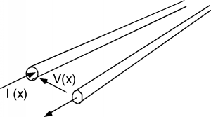Figure \(\PageIndex{1}\): "Generic" transmission line

The generic line consists of two conductors. We will suppose a potential difference \(V(x)\) exists between the two conductors, and that a current \(I(x)\) flows down one conductor, and returns via the other. For the time being, we will let the transmission line be "semi-infinite", which means we have access to the line at some point \(x\), but the line then extends out in the \(x\) direction to infinity. (Such lines are a bit difficult to handle in the lab!)

In order to be able to describe how \(V(x)\) and \(I(x)\) behave on this line, we have to make some kind of model of the electrical characteristics of the line itself. We cannot just make up any model we want, however; we have to base the model on physical realities.

Let's start out by just considering one of the conductors and the physical effects of current flowing though that conductor. We know from freshman physics that a current flowing in a wire gives rise to a magnetic field, \(H\) (Figure \(\PageIndex{2}\)). Multiply \(H\) by \(\mu\) and you get \(B\), the magnetic flux density, and then integrate \(B\) over a plane parallel to the wires and you get \(\Phi\), the magnetic flux "linking" the circuit. This is shown in Figure \(\PageIndex{3}\) for at least part of the surface. The definition of \(L\), the inductance of a circuit element, is just \[L = \frac{\Phi}{I}\]

where \(\Phi\) is the flux linking the circuit element, and \(I\) is the current flowing through it. Our only problem in finding \(\Phi\) is that the longer a section of wire we take, the more \(\Phi\) we have for the same \(I\). Thus, we will introduce the concept of a distributed parameter.

Definition: Distributed Parameter

A distributed parameter is a parameter which is spread throughout a structure and is not confined to a lumped element such as a coil of wire.

For instance, we will hereby define \(\mathbf{L}\) as the distributed inductance for the transmission line. It has units of \(\mathrm{Henrys} / \mathrm{meter}\). If we have a length of transmission line \(x_{0}\) meters long, and if that line has a distributed inductance of \(\mathbf{L} \mathrm{~H} / \mathrm{m}\), then the inductance \(L\) of that length of line is just \(L = \mathbf{L} x_{0}\).

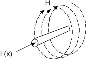Figure \(\PageIndex{2}\): Buildup of magnetic field

Likewise, if we have two conductors separated by some distance, and if there is a potential difference \(V\) between the conductors, then there must be some charge \(\pm (Q)\) on the two conductors which gives rise to that potential difference. We can imagine a linear charge distribution on the transmission line, \(\rho\) (in units of \(\mathrm{C} / \mathrm{m}\)), where we have \(\rho \mathrm{~Coulombs} / \mathrm{m}\) on one conductor, and \(-\rho \mathrm{~Coulombs} / \mathrm{m}\) on the other conductor. For a line of length \(x_{0}\), we would have \(Q = \pm \left(\rho x_{0}\right)\) on each section of wire. Whenever you have two charged conductors with a voltage difference between them, you can describe the ratio of the charge to the voltage as a capacitance. The two conductors would have a capacitance \[\begin{array}{l} C &= \frac{Q}{V} \\ &= \frac{\rho x_{0}}{V} \end{array}\]

and a distributed capacitance \(\mathbf{C}\) (in units of \(\mathrm{Farads} / \mathrm{m}\)), which is just \(\frac{\rho}{V}\). A length of line \(x_{0}\) long would have a capacitance \(C = \mathbf{C} x_{0} \mathrm{~Farads}\) associated with it, as in Figure \(\PageIndex{4}\).

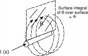Figure \(\PageIndex{3}\): Find the flux linkage \(\Phi\)

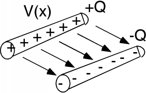Figure \(\PageIndex{4}\): Line capacitance

Thus, we see that the transmission line has both a distributed inductance \(\mathbf{L}\) and a distributed capacitance \(\mathbf{C}\), which are tied up with each other. There is really no way in which we can separate one from the other. In other words, we cannot have only the capacitance, or only the inductance'; there will always be some of each associated with each section of line now matter how small or how big we make it.

We are now ready to build our model. What we want to do is to come up with some arrangement of inductors and capacitors which will represent electrically the properties of the distributed capacitance and inductance we discussed above. As a length of line gets longer, its capacitance increases, so we had better put the distributed capacitances in parallel with one another, since that is the way capacitors add up. Also, as the line gets longer, its total inductance increases, so we had better put the distributed inductances in series with one another, for that is the way inductances add up. Figure \(\PageIndex{5}\) is a representation of the distributed inductance and capacitance of the generic transmission line.

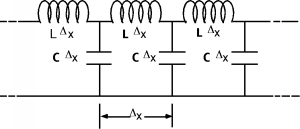Figure \(\PageIndex{5}\): Distributed parameter model

We break the line up into sections \(\Delta x\) long, each one with an inductance \(\mathbf{L} \Delta x\) and a capacitance \(\mathbf{C} \Delta x\). If we halve \(\Delta x\), we would halve the inductance and capacitance of each section, but we'd have twice as many of them per unit length. Duh! The point is no matter how fine we make \(\mathbf{C} \Delta x\), we still have inductors and capacitors arranged like we see in Figure \(\PageIndex{5}\), with the two kinds of components intermixed.

We could make a more realistic model and realize that all real wires have series resistance associated with them, and that whatever we use to keep the two conductors separated will have some leakage conductance associated it. To account for this we would introduce a series resistance \(\mathbf{R}\) (\(\Omega\) per unit length) and a series conductance \(\mathbf{G}\) (\(\Omega\) per unit length). One section of our line model then looks like Figure \(\PageIndex{6}\).

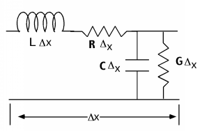Figure \(\PageIndex{6}\): Complete distributed model

Although this is a more realistic model, it leads to much more complicated math. We will start out anyway, ignoring the series resistance \(\mathbf{R}\) and the shunt conductance \(\mathbf{G}\). This "approximation" turns out to be pretty good as long as either the line is not too long, or the frequencies of the signals we are sending down the line do not get too high. Without the series resistance or parallel conductance we have what is called an ideal lossless transmission line.