5.3: Transmission Line Equation

We need to solve the telegrapher's equations, \[\frac{\partial V(x, t)}{\partial x} = -\left(\mathbf{L} \frac{\partial I(x, t)}{\partial t}\right)\] \[\frac{\partial (I, t)}{\partial x} = - \left(\mathbf{C} \frac{\partial V(x, t)}{\partial t}\right)\]

The way we will proceed to a solution, and the way you always proceed when confronted with a pair of equations such as these, is to take a spatial derivative of one equation, and then substitute the second equation in for the spatial derivative in the first and you end up with...well, let's try it and see.

Taking a derivative with respect to \(x\) of Equation \(\PageIndex{1}\), \[\frac{\partial^{2} V(x, t)}{\partial x_{2}^{2}} = -\left(\mathbf{L} \frac{\partial^{2} I(x, t)}{\partial t \partial x}\right)\]

Now we substitute in for \(\frac{\partial I(x, t)}{\partial x}\) from Equation \(\PageIndex{2}\): \[\frac{\partial^{2} V(x, t)}{\partial x_{2}^{2}} = \mathbf{LC} \frac{\partial^{2} V(x, t)}{\partial t_{2}^{2}}\]

It should be very easy for you to derive \[\frac{\partial^{2} I(x, t)}{\partial x_{2}^{2}} = \mathbf{LC} \frac{\partial^{2} I(x, t)}{\partial t_{2}^{2}}\]

Oh, I know you all love differential equations! Well, let's take a look at these and just think for a minute. For either \(V(x, t)\) or \(I(x, t)\), we need to find a function that has some rather stringent requirements. First of all, the function must be of the form such that no matter whether we take its second derivative in space (\(x\)) or in time (\(t\)), it must end up differing in the way it behaves in \(x\) or \(t\) by no more than just a constant (\(\mathbf{LC}\)).

In fact, we can be more specific than that. First, \(V(x, t)\) must have the same functional form for both its \(x\) and \(t\) variation. At most, the two derivatives must differ only by a constant. Let's try a "lucky" guess and let: \[V(x, t) = V_{0} f(x - vt)\]

where \(V_{0}\) is the amplitude of the voltage, and \(f\) is some function of a form yet undetermined. Well, \[\frac{\partial f(x - vt)}{\partial t} = -(vf')\]

and \[\frac{\partial^{2} f(x-vt)}{\partial t_{2}^{2}} = v^{2} \frac{\text{d} f}{\text{d}}\]

Note also, that \[\frac{\partial^{2} f(x-vt)}{\partial x_{2}^{2}} = f''\]

Now, let's take Equations \(\PageIndex{6}\), \(\PageIndex{8}\), and \(\PageIndex{9}\) and substitute them into Equation \(\PageIndex{4}\): \[V_{0} \frac{\text{d} f}{\text{d}} = \mathbf{LC} V_{0} v^{2} \frac{\text{d} f}{\text{d}}\]

Our "lucky" guess works as a solution as long as \[v = \pm \frac{1}{\sqrt{\mathbf{LC}}}\]

So, what is this \(f(x - vt)\)? We don't know yet what its actual functional form will be, but suppose at some point in time, \(t_{1}\), the function looks like Figure \(\PageIndex{1}\).

Figure \(\PageIndex{1}\): \(f(x)\) at time \(t_{1}\)

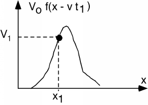
At point \(x_{1}\), the function takes on the value \(V_{1}\). Now, let's advance to time \(t_{2}\). We look at the function and we see Figure \(\PageIndex{2}\).

Figure \(\PageIndex{2}\): \(f(x)\) at a later time \(t_{2}\)

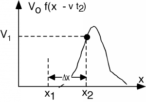
If \(t\) increases from \(t_{1}\) to \(t_{2}\), then \(x\) will have to increase from \(x_{1}\) to \(x_{2}\) in order for the argument of \(f\) to have the same value, \(V_{1}\). Thus we find \[x_{1} - vt_{1} \equiv x_{2} - vt_{2}\]

which can be re-written as \[\frac{x_{2}-x_{1}}{t_{2}-t_{1}} = \frac{\Delta (x)}{\Delta (t)} \equiv v_{p} = \frac{1}{\sqrt{\mathbf{LC}}}\]

where \(v_{p}\) is the velocity with which the function is moving along the x-axis! (We use the subscript "p" to indicated that what we have here is what is called the phase velocity. We will encounter another velocity called the group velocity a little later in the course.)

If we had "guessed" an \(f(x + vt)\) for our function, it should be pretty easy to see that this would have given us a signal moving in the minus \(x\) direction, instead of the plus \(x\) direction. Thus we shall denote \[V_{\text{plus}} = V^{+} f \left(x - \frac{1}{\sqrt{\mathbf{LC}}} t\right)\]

the positive-going voltage function and \[V_{\text{minus}} = V^{-} f\left(x + \frac{1}{\sqrt{\mathbf{LC}}} t\right)\]

the negative-going voltage function. Notice that since we are taking the second derivative of \(f\) with respect to \(t\), we are free to choose either a \(\frac{1}{\sqrt{\mathbf{LC}}}\) or a \(- \frac{1}{\sqrt{\mathbf{LC}}}\) in front of the time argument inside \(f\). Also note that these are our only choices for a solution. As we know from Differential Equations, a second order equation has, at most, two independent solutions.

Since \(I(x, t)\) has the same differential equation describing its behavior, the solutions for \(I\) must also be of the exact same form. Thus we can let \[I_{\text{plus}} = I^{+} f \left(x - \frac{1}{\sqrt{\mathbf{LC}}} t\right)\] represent the current function which goes in the positive \(x\) direction, and \[I_{\text{minus}} = I^{-} f \left(x + \frac{1}{\sqrt{\mathbf{LC}}} t\right)\] represent the negative going current function.

Now, let's take Equation \(\PageIndex{16}\) and Equation \(\PageIndex{14}\) and substitute them into Equation \(\PageIndex{1}\): \[\frac{V^{+}}{\sqrt{\mathbf{LC}}} f \left(x - \frac{1}{\sqrt{\mathbf{LC}}} t\right) = \mathbf{L} I^{+} f \left(x - \frac{1}{\sqrt{\mathbf{LC}}} t\right)\]

This can be solved for \(V^{+}\) in terms of \(I^{+}\). \[V^{+} = \sqrt{\frac{\mathbf{L}}{\mathbf{C}}} \ I^{+} \equiv Z_{0} I^{+}\]

where \(Z_{0} = \sqrt{\frac{\mathbf{L}}{\mathbf{C}}}\) is called the characteristic impedance of the transmission line. We will leave it as an exercise to the reader to ensure that indeed \(\sqrt{\frac{\mathbf{L}}{\mathbf{C}}}\) has units of Ohms. For practice, and understanding about just how these equations work, the reader should ensure themselves that

\[V^{-} = -\left( \sqrt{\frac{\mathbf{L}}{\mathbf{C}}} I^{-}\right) \equiv -\left(Z_{0} I^{-}\right)\]

Note the "subtle" difference here, with the presence of a minus sign in front of the RHS of the equation!

We've been through lots of equations recently, so it is probably worth our while to summarize what we know so far.

1. The telegrapher's equations allow two solutions for the voltage and current on a transmission line. One moves in the \(x\) direction and the other moves in the \(-x\) direction.
2. Both signals move at a constant velocity \(v_{p}\) given by Equation \(\PageIndex{21}\).
3. The voltage and current signals are related to one another by the characteristic impedance \(Z_{0}\), which is found with Equation \(\PageIndex{22}\)

\[v_{p} = \frac{1}{\sqrt{\mathbf{LC}}}\] \[Z_{0} = \sqrt{\frac{\mathbf{L}}{\mathbf{C}}}\] \[\frac{V^{+}}{I^{+}} = Z_{0}\] \[\frac{V^{-}}{I^{-}} = -Z_{0}\]