12.2: The Sampling Theorem

Last updated
Save as PDF

Page ID: 3622

\( \newcommand{\vecs}[1]{\overset { \scriptstyle \rightharpoonup} {\mathbf{#1}} } \) \( \newcommand{\vecd}[1]{\overset{-\!-\!\rightharpoonup}{\vphantom{a}\smash {#1}}} \)\(\newcommand{\id}{\mathrm{id}}\) \( \newcommand{\Span}{\mathrm{span}}\) \( \newcommand{\kernel}{\mathrm{null}\,}\) \( \newcommand{\range}{\mathrm{range}\,}\) \( \newcommand{\RealPart}{\mathrm{Re}}\) \( \newcommand{\ImaginaryPart}{\mathrm{Im}}\) \( \newcommand{\Argument}{\mathrm{Arg}}\) \( \newcommand{\norm}[1]{\| #1 \|}\) \( \newcommand{\inner}[2]{\langle #1, #2 \rangle}\) \( \newcommand{\Span}{\mathrm{span}}\) \(\newcommand{\id}{\mathrm{id}}\) \( \newcommand{\Span}{\mathrm{span}}\) \( \newcommand{\kernel}{\mathrm{null}\,}\) \( \newcommand{\range}{\mathrm{range}\,}\) \( \newcommand{\RealPart}{\mathrm{Re}}\) \( \newcommand{\ImaginaryPart}{\mathrm{Im}}\) \( \newcommand{\Argument}{\mathrm{Arg}}\) \( \newcommand{\norm}[1]{\| #1 \|}\) \( \newcommand{\inner}[2]{\langle #1, #2 \rangle}\) \( \newcommand{\Span}{\mathrm{span}}\)\(\newcommand{\AA}{\unicode[.8,0]{x212B}}\)

There are many different ways in which an analog signal may be turned into a digital form. This process is referred to as AD conversion or, more simply, as digitization. We will only examine the most popular method, called pulse code modulation, or PCM for short. The reverse of this process, or turning the digital information back into analog form, is called DA conversion. The two most important charracteristics in the conversion process are sampling frequency and amplitude resolution. Let's look at the basic idea behind PCM.

In essence, PCM measures and encodes the value of the input signal at specific points in time. Normally, the time spacing is constant, and several points are used over the length of one input cycle. In other words, the process involves taking representative samples of the input signal over time. This is shown graphically in Figure \(\PageIndex{1}\), and is referred to as sampling. The result of the sampling procedure is a list of times and corresponding amplitude values. A sequence might look something like: at \(t = 1\) ms, \(V_{in} = 23\) mV; at \(t = 2\) ms, \(V_{in} = 45\) mV; at \(t = 3\) ms, \(V_{in} = −15\) mV; etc. If the time interval between samples is held constant (i.e., constant rate of sampling), then all we need to know is a starting time and the sampling rate in order to reconstruct the actual sample times¹. This is much more efficient than recording each sample time. The resulting amplitude values may be manipulated in a variety of ways since they are now in a numeric form. The ultimate accuracy of this conversion will depend on two primary factors: how often we sample the signal and the accuracy and resolution of the sample measurement. Theoretically, the conversion will never be 100% accurate; that is, once converted, a finite amount of information will be lost forever. Another way of stating this is that when the digital representation is converted back to analog, the result will not be identical to the original waveform. In practical terms, it is possible to reduce the error to such small values that it may be ignored in many applications. It is important then, that we investigate the implications of sample rate and accuracy/resolution on the quality of conversion.

12.2.1.png

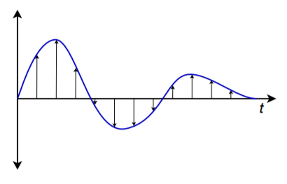
Figure \(\PageIndex{1}\): Sampling input signals over time.

References

¹The terms sample rate and sample frequency are often used interchangeably, and are usually denoted by \(f_s\).