3.8: Exercises

Last updated
Save as PDF

Page ID: 41105

\( \newcommand{\vecs}[1]{\overset { \scriptstyle \rightharpoonup} {\mathbf{#1}} } \) \( \newcommand{\vecd}[1]{\overset{-\!-\!\rightharpoonup}{\vphantom{a}\smash {#1}}} \)\(\newcommand{\id}{\mathrm{id}}\) \( \newcommand{\Span}{\mathrm{span}}\) \( \newcommand{\kernel}{\mathrm{null}\,}\) \( \newcommand{\range}{\mathrm{range}\,}\) \( \newcommand{\RealPart}{\mathrm{Re}}\) \( \newcommand{\ImaginaryPart}{\mathrm{Im}}\) \( \newcommand{\Argument}{\mathrm{Arg}}\) \( \newcommand{\norm}[1]{\| #1 \|}\) \( \newcommand{\inner}[2]{\langle #1, #2 \rangle}\) \( \newcommand{\Span}{\mathrm{span}}\) \(\newcommand{\id}{\mathrm{id}}\) \( \newcommand{\Span}{\mathrm{span}}\) \( \newcommand{\kernel}{\mathrm{null}\,}\) \( \newcommand{\range}{\mathrm{range}\,}\) \( \newcommand{\RealPart}{\mathrm{Re}}\) \( \newcommand{\ImaginaryPart}{\mathrm{Im}}\) \( \newcommand{\Argument}{\mathrm{Arg}}\) \( \newcommand{\norm}[1]{\| #1 \|}\) \( \newcommand{\inner}[2]{\langle #1, #2 \rangle}\) \( \newcommand{\Span}{\mathrm{span}}\)\(\newcommand{\AA}{\unicode[.8,0]{x212B}}\)

Reduce the following signal flow graph to two edges and three nodes. That is, write down the expression for \(b_{2}\) in terms of \(a_{1}\) and \(a_{2}\), eliminating the variables \(x_{1},\: x_{2},\) and \(x_{3}\).

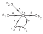
Figure \(\PageIndex{1}\)

Reduce the following signal flow graph to one edge and two nodes. That is, write down the expression for \(b_{2}\) in terms of \(a_{1}\), eliminating the variables \(x_{1}\) and \(x_{2}\).

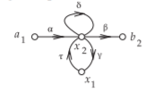
Figure \(\PageIndex{2}\)

The scattering parameters of a two-port are \(S_{11} = 0.25,\: S_{12} = 0,\: S_{21} = 1.2,\) and \(S_{22} = 0.5\). The system reference impedance is \(50\:\Omega\) and the Thevenin equivalent impedance of the source at Port \(\mathsf{1}\) is \(Z_{G} = 50\:\Omega\). The power available from the source connected to Port \(\mathsf{1}\) is \(1\text{ mW}\). The load impedance is \(Z_{L} = 25\:\Omega\). Using SFGs, determine the power dissipated by the load at Port \(\mathsf{2}\).

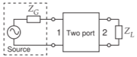
Figure \(\PageIndex{3}\)

Draw the SFG of a two-port with a load at Port \(\mathsf{2}\) having a voltage reflection coefficient of \(\Gamma_{L}\), and at Port \(\mathsf{1}\) a source reflection coefficient of \(\Gamma_{S}\). \(\Gamma_{S}\) is the reflection coefficient looking from Port \(\mathsf{1}\) of the two-port toward the generator. Keep the \(S\) parameters of the two-port in symbolic form (e.g., \(S_{11},\: S_{12},\: S_{21},\) and \(S_{22}\)). Using SFG analysis, derive an expression for the reflection coefficient looking into the two-port at Port \(\mathsf{2}\). You must show the stages in collapsing the SFG to the minimal form required.
A three-port has the scattering parameters:
\[\left[\begin{array}{ccc}{0}&{\gamma}&{\delta}\\{\alpha}&{0}&{\epsilon}\\{\theta}&{\beta}&{0}\end{array}\right]\nonumber \]
Port \(\mathsf{2}\) is terminated in a load with a reflection coefficient \(\Gamma_{L}\). Reduce the three-port to a two-port using signal flow graph theory. Write down the four scattering parameters of the final two-port.
The \(50-\Omega\: S\) parameters of a three-port are
\[\left[\begin{array}{lll}{0.2\angle 180^{\circ}}&{0.8\angle -45^{\circ}}&{0.1\angle 45^{\circ}} \\ {0.8\angle -45^{\circ}}&{0.2\angle 0^{\circ}}&{0.1\angle 90^{\circ}} \\ {0.1\angle 45^{\circ}}&{0.1\angle 90^{\circ}}&{0.1\angle 180^{\circ}}\end{array}\right]\nonumber \]
1. Is the three-port reciprocal? Explain your answer.
2. Write down the criteria for a network to be lossless.
3. Is the three-port lossless? You must show your work.
4. Draw the SFG of the three-port.
5. A \(50\:\Omega\) load is attached to Port \(\mathsf{3}\). Use SFG operations to derive the SFG of the two-port with just Ports \(\mathsf{1}\) and \(\mathsf{2}\). Write down the two-port \(S\) parameter matrix.
The \(50\:\Omega\: S\) parameters of a three-port are
\[\left[\begin{array}{lll}{0.2\angle 180^{\circ}}&{0.8\angle -45^{\circ}}&{0.1\angle 45^{\circ}}\\{0.8\angle -45^{\circ}}&{0.2\angle 0^{\circ}}&{0.1\angle 90^{\circ}} \\ {0.1\angle 45^{\circ}}&{0.1\angle 90^{\circ}}&{0.1\angle 180^{\circ}}\end{array}\right]\nonumber \]
1. Is the three-port reciprocal? Explain.
2. Write down the criteria for a network to be lossless.
3. Is the three-port lossless? Explain.
4. Draw the SFG of the three-port.
5. A \(150\:\Omega\) load is attached to Port \(\mathsf{3}\). Derive the SFG of the two-port with just Ports \(\mathsf{1}\) and \(\mathsf{2}\). Write down the two-port \(S\) parameter matrix of the simplified network.
A system consists of \(\mathsf{2}\) two-ports in cascade. The \(S\)-parameter matrix of the first two-port is \(\mathbf{S}_{A}\) and the \(S\) parameter matrix of the second two-port is \(\mathbf{S}_{B}\). The second two-port is terminated in a load with a reflection coefficient \(\Gamma_{L}\). (Just to be clear, \(\mathbf{S}_{A}\) is followed by \(\mathbf{S}_{B}\), which is then terminated in \(\Gamma_{L}\). Port \(\mathsf{2}\) of \(\mathbf{S}_{A}\) is connected to Port \(\mathsf{1}\) of \([S_{B}]\).) The individual \(S\) parameters of the two-ports are as follows:
\[\mathbf{S}_{A}=\left[\begin{array}{cc}{a}&{c}\\{c}&{b}\end{array}\right]\quad\text{and}\quad\mathbf{S}_{B}=\left[\begin{array}{cc}{d}&{f}\\{f}&{e}\end{array}\right]\nonumber \]
1. Draw the SFG of the system consisting of the two cascaded two-ports and the load.
2. Ignoring the load, is the cascaded two-port system reciprocal? If there is not enough information to decide, then say so. Give your reasons.
3. Ignoring the load, is the cascaded two-port system lossless? If there is not enough information to decide, then say so. Give your reasons.
4. Consider that the load has no reflection (i.e., \(\Gamma_{L} = 0\)). Use SFG analysis to find the input reflection coefficient looking into Port \(\mathsf{1}\) of \([S_{A}]\). Your answer should be \(\Gamma_{\text{in}}\) in terms of \(a, b,\ldots , f\).
A circulator is a three-port device that is not reciprocal and selectively shunts power from one port to another. The \(S\) parameters of an ideal circulator are
\[ [S]=\left[\begin{array}{ccc}{0}&{1}&{0}\\{0}&{0}&{1}\\{1}&{0}&{0}\end{array}\right]\nonumber \]
1. Draw the three-port and discuss power flow.
2. Draw the SFG of the circulator.
3. If Port \(\mathsf{2}\) is terminated in a load with reflection coefficient \(0.2\), reduce the SFG of the circulator to a two-port with Ports \(\mathsf{1}\) and \(\mathsf{3}\) only.
4. Write down the \(2\times 2\: S\) parameter matrix of the (reduced) two-port.
The \(S\) parameters of a certain two-port are \(S_{11} = 0.5 +\jmath 0.5,\: S_{21} = 0.95 +\jmath 0.25,\: S_{12} = 0.15 −\jmath 0.05,\: S_{22} = 0.5 −\jmath 0.5\). The system reference impedance is \(50\:\Omega\).
1. Is the two-port reciprocal?
2. Which of the following is a true statement about the two-port?
  1. It is unitary.
  2. Overall power is produced by the two-port.
  3. It is lossless.
  4. If Port \(\mathsf{2}\) is matched, then the real part of the input impedance (at Port \(\mathsf{1}\)) is negative.
  5. A and C.
  6. A and B.
  7. A, B, and C
  8. None of the above.
3. What is the value of the load required for maximum power transfer at Port \(\mathsf{2}\)? Express your answer as a reflection coefficient.
4. Draw the SFG for the two-port with a load at Port \(\mathsf{2}\) having a voltage reflection coefficient of \(\Gamma_{L}\) and at Port \(\mathsf{1}\) a source reflection coefficient of \(\Gamma_{S}\).
The \(50-\Omega\: S\) parameters of a three-port are
\[\left[\begin{array}{ccc}{0.2}&{0.8}&{0.1}\\{0.8}&{0.2}&{0.1}\\{0.1}&{0.1}&{0.1}\end{array}\right]\nonumber \]
1. Is the three-port reciprocal? Explain your answer.
2. Write down the criteria for a network to be lossless.
3. Is the three-port lossless? You must show your work.
4. Draw the SFG of the three-port.
5. A \(50\:\Omega\) load is attached to Port \(\mathsf{3}\). Use SFG operations to derive the SFG of the two-port with just Ports \(\mathsf{1}\) and \(\mathsf{2}\). Write down the two-port \(S\) parameter matrix.
The \(50-\Omega\: S\) parameters of a three-port are
\[\left[\begin{array}{ccc}{0.5}&{0.4}&{0.5}\\{0.6}&{0.5}&{0.5}\\{0.5}&{0.5}&{0.5}\end{array}\right]\nonumber \]
1. Is the three-port reciprocal? Explain.
2. Write down the criteria for a network to be lossless.
3. Is the three-port lossless? Explain.
4. Draw the SFG of the three-port.
5. A \(150\:\Omega\) load is attached to Port \(\mathsf{3}\). Derive the SFG of the two-port with just Ports \(\mathsf{1}\) and \(\mathsf{2}\). Write down the two-port \(S\) parameter matrix.
In the distribution of signals on a cable TV system a \(75-\Omega\) coaxial cable is used, with a loss of \(0.1\text{ dB/m}\) at \(1\text{ GHz}\). If a subscriber disconnects a television set from the cable so that the load impedance looks like an open circuit, estimate the input impedance of the cable at \(1\text{ GHz}\) and \(1\text{ km}\) from the subscriber. An answer within \(1\%\) is required. Estimate the error of your answer. Indicate the input impedance on a Smith chart, drawing the locus of the input impedance as the line is increased in length from nothing to \(1\text{ km}\). (Consider that the dielectric filling the line has \(\epsilon_{r} = 1\).)
A resistive load has a reflection coefficient with a magnitude of \(0.7\). If a transmission line is placed in series with the load, on a polar plot sketch the locus of the input reflection coefficient looking into the input of the terminated line as the line increases in electrical length from zero to \(\lambda /2\). By reading the Smith chart, determine the normalized input impedance of the line when it has an electrical length of \(\pi /2\).
A complex load has a reflection coefficient of \(0.5+\jmath 0.5\). If a transmission line is placed in series with the load, on a polar plot sketch the locus of the input reflection coefficient looking into the input of the terminated line as the line increases in electrical length from zero to \(\pi /2\).
A resistive load has a reflection coefficient of \(−0.5\). If a transmission line is placed in series with the load, on a polar plot sketch the locus of the input reflection coefficient looking into the input of the terminated line as the line increases in electrical length from \(0\) to \(3\lambda /8\).
\(S_{21}\) of a two-port is \(0.5\). If a transmission line is placed in series with Port \(\mathsf{1}\), on a polar plot sketch the locus of \(S_{21}\) of the augmented two-port as the electrical length of the line increases from zero to \(\lambda /2\).
A load has an impedance \(Z = 115 −\jmath 20\:\Omega\).
1. What is the reflection coefficient, \(\Gamma_{L}\), of the load in a \(50\:\Omega\) reference system?
2. Plot the reflection coefficient on a polar plot of reflection coefficient.
3. If a one-eighth wavelength long lossless \(50-\Omega\) transmission line is connected to the load, what is the reflection coefficient, \(\Gamma_{\text{in}}\), looking into the transmission line? (Again, use the \(50\:\Omega\) reference system.) Plot \(\Gamma_{\text{in}}\) on the polar reflection coefficient plot of part (b). Clearly identify \(\Gamma_{\text{in}}\) and \(\Gamma_{L}\) on the plot.
4. On the Smith chart, identify the locus of \(\Gamma_{\text{in}}\) as the length of the transmission line increases from \(0\) to \(\lambda /8\) long. That is, on the Smith chart, plot \(\Gamma_{\text{in}}\) as the length of the transmission line varies.
A load has a reflection coefficient with a magnitude of \(0.5\). If a transmission line is placed in series with the load, on a polar plot sketch the locus of the input reflection coefficient looking into the input of the terminated line as the line increases in electrical length from zero to \(\lambda /2\). What is the normalized input impedance of the line when it has an electrical length of \(\lambda /2\)?
A resistive load has a reflection coefficient with a magnitude of \(0.7\). If a transmission line is placed in series with the load, on a polar plot sketch the locus of the input reflection coefficient looking into the input of the terminated line as the line increases in electrical length from zero to \(\lambda /4\). By reading the Smith chart, determine the normalized input impedance of the line when it has an electrical length of \(\lambda /4\). Problems 21 to 27 refer to the normalized Smith chart in Figure \(\PageIndex{7}\) with reference impedance \(Z_{\text{REF}} = 50\:\Omega\) and reflection coefficient \(\Gamma\), voltage reflection coefficient \(^{V}\Gamma\), current reflection coefficient \(^{I}\Gamma\), and normalized impedance \(z = r+\jmath x\) and admittance \(y = g +\jmath b\). \(\Gamma\) should be given in magnitude-angle format.
1. What is \(^{V}\Gamma\) at \(\mathsf{A}\)?
2. What is \(^{I}\Gamma\) at \(\mathsf{A}\)?
3. What is \(r\) at \(\mathsf{B}\)?
4. What is \(z\) at \(\mathsf{C}\)?
5. What is \(y\) at \(\mathsf{D}\)?
6. What is \(|\Gamma |\) at \(\mathsf{F}\)?
7. What is \(b\) at \(\mathsf{I}\)?
8. What is \(\Gamma\) at \(\mathsf{P}\)?
9. What is \(\Gamma\) at \(\mathsf{D}\)?
10. What is \(\Gamma\) at \(\mathsf{T}\)?
1. What is \(z\) at \(\mathsf{A}\)?
2. What is \(y\) at \(\mathsf{I}\)?
3. What is \(z\) at \(\mathsf{E}\)?
4. What is \(y\) at \(\mathsf{Z}\)?
5. What is \(y\) at \(\mathsf{H}\)?
6. What is \(|\Gamma |\) at \(\mathsf{W}\)?
7. What is \(b\) at \(\mathsf{F}\)?
8. What is \(x\) at \(\mathsf{K}\)?
9. What is \(\Gamma\) at \(\mathsf{K}\)?
10. What is \(\Gamma\) at \(\mathsf{R}\)?
1. What is \(y\) at \(\mathsf{A}\)?
2. What is \(y\) at \(\mathsf{I}\)?
3. What is \(z\) at \(\mathsf{G}\)?
4. What is \(y\) at \(\mathsf{O}\)?
5. What is \(y\) at \(\mathsf{V}\)?
6. What is \(\Gamma\) at \(\mathsf{B}\)?
7. What is \(x\) at \(\mathsf{C}\)?
8. What is \(\Gamma\) at \(\mathsf{G}\)?
9. What is \(z\) at \(\mathsf{L}\), label this \(z_{L}\)?
10. Use the Smith chart to find \(z_{\text{in}}\) of a \(50\:\Omega\:\lambda /8\)-long line with load \(z_{L}\)?
1. What is \(^{V}\Gamma\) at \(\mathsf{M}\)?
2. What is \(^{I}\Gamma\) at \(\mathsf{M}\)?
3. What is \(r\) at \(\mathsf{W}\)?
4. What is \(z\) at \(\mathsf{Y}\)?
5. What is \(y\) at \(\mathsf{V}\)?
6. What is \(|\Gamma |\) at \(\mathsf{B}\)?
7. What is \(b\) at \(\mathsf{K}\)?
8. What is \(\Gamma\) at \(\mathsf{V}\)?
9. What is \(\Gamma\) at \(\mathsf{P}\)?
10. What is \(\Gamma\) at \(\mathsf{N}\)?
1. What is \(z\) at \(\mathsf{M}\)?
2. What is \(y\) at \(\mathsf{K}\)?
3. What is \(z\) at \(\mathsf{S}\)?
4. What is \(y\) at \(\mathsf{R}\)?
5. What is \(g\) at \(\mathsf{B}\)?
6. What is \(|\Gamma |\) at \(\mathsf{F}\)?
7. What is \(b\) at \(\mathsf{B}\)?
8. What is \(x\) at \(\mathsf{I}\)?
9. What is \(\Gamma\) at \(\mathsf{I}\)?
10. What is \(\Gamma\) at \(\mathsf{Q}\)?
1. What is \(g\) at \(\mathsf{M}\)?
2. What is \(r\) at \(\mathsf{K}\)?
3. What is \(y\) at \(\mathsf{S}\)?
4. What is \(z\) at \(\mathsf{R}\)?
5. What is \(y\) at \(\mathsf{Z}\)?
6. What is \(\Gamma\) at \(\mathsf{W}\)?
7. What is \(x\) at \(\mathsf{Y}\)?
8. What is \(\Gamma\) at \(\mathsf{T}\)?
9. What is \(z\) at \(\mathsf{O}\), label this \(z_{O}\)?
10. Using the Smith chart find \(z_{\text{in}}\) of a \(3\lambda /8\)- long \(50\:\Omega\) line with load \(z_{O}\)?
1. What is \(g\) at \(\mathsf{P}\)?
2. What is \(y\) at \(\mathsf{J}\)?
3. What is \(\Gamma\) at \(\mathsf{L}\)?
4. What is \(z\) at \(\mathsf{N}\)?
5. What is \(y\) at \(\mathsf{S}\)?
6. What is \(|\Gamma |\) at \(\mathsf{U}\)?
7. What is \(^{V}\Gamma\) at \(\mathsf{X}\)?
8. What is \(^{I}\Gamma\) at \(\mathsf{X}\)?
9. What is \(g\) at \(\mathsf{B}\)?
10. What is \(x\) at \(\mathsf{I}\)?
Design a short-circuited stub to realize a normalized susceptance of \(2.15\). Show the locus of the stub as its length increases from zero to its final length. What is the minimum length of the stub in terms of wavelengths?
Design a short-circuited stub to realize a normalized susceptance of \(−0.56\). Show the locus of the stub as its length increases from zero to its final length. What is the minimum length of the stub in terms of wavelengths?
Design a short-circuited stub to realize a normalized susceptance of \(−2.2\). Show the locus of the stub as its length increases from zero to its final length. What is the minimum length of the stub in terms of wavelengths?
A \(75-\Omega\) transmission line is terminated in a load with a reflection coefficient, \(\Gamma\), normalized to \(75\:\Omega\), of \(0.5\angle 45^{\circ}\). If \(\Gamma\) at the input of the line is \(0.5\angle −135^{\circ}\), what is the minimum electrical length of the line in degrees.
An open-circuited \(75-\Omega\) transmission line has an input reflection coefficient with an angle of \(40^{\circ}\) what is the electrical length of the line in degrees? If there is more than one answer provide at least two correct answers.
Use a Smith chart to design a microstrip network to match a load \(Y_{L} = 28 −\jmath 12\text{ mS}\) to a source \(Y_{S} = 6+\jmath 12\text{ mS}\). Use transmission lines only and use short-circuited stubs. Use a reference impedance of \(50\:\Omega\).
1. Draw the matching network problem labeling source and load admittances and labeling the admittance looking into the matching network from the source as \(Y_{1}\).
2. What is the condition for maximum power transfer at the source side of the matching network in terms of admittances?
3. What is the condition for maximum power transfer at the source side of the matching network in terms of reflection coefficients?
4. What is the reference admittance \(Y_{\text{REF}}\)?
5. What is the value of the normalized source admittance?
6. What is the value of the normalized load admittance?
7. On a Smith chart (not a sketch) identify, i.e. draw, the electrical designs of two suitable matching networks. Identify the designs using the labels \(\text{D}1\) and \(\text{D}2\) on the loci.
8. Develop the complete electrical design of a matching network using the Smith chart using \(50\:\Omega\) lines only. You only need do one design.
9. Draw the microstrip layout of the matching network and identify critical parameters such characteristic impedances and electrical length. Ensure that you identify which is the source side and which is the load side. You do not need to determine the widths of the lies or their physical lengths.
Repeat Exercise 33 with \(Y_{L} = 20 +\jmath 20\text{ mS}\) to a source \(Y_{S} =4+\jmath 20\text{ mS}\).
Repeat Example 3.4.1 using the full impedance Smith chart of Figure 3.4.1.
Plot the normalized impedances \(z_{A} = 0.5+\jmath 0.5,\: z_{A} = 0.5 +\jmath 0.5,\) and \(z_{B} = 0.185 −\jmath 1.05\) on the full impedance Smith chart of Figure 3.4.1. [Parallels Example 3.4.1]

In Figure \(\PageIndex{4}\) the results of several different experiments are plotted on a Smith chart. Each experiment measured the input reflection coefficient from a low frequency (denoted by a circle) to a high frequency (denoted by a square) of a one-port. Determine the load that was measured. The loads that were measured are one of those shown below.

Load	Description
i	An inductor
ii	A capacitor
iii	A reactive load at the end of a transmission line
iv	A resistive load at the end of a transmission line
v	A parallel connection of an inductor, a resistor, and a capacitor going through resonance and with a transmission line offset
vi	A series connection of a resistor, an inductor and a capacitor going through resonance and with a transmission line offset
vii	A series resistor and inductor
viii	An unknown load and not one of the above

Table \(\PageIndex{1}\)
For each of the measurements below indicate the load or loads using the load identifier above (e.g., i, ii, etc.).

What load(s) is indicated by curve \(\mathsf{A}\)?
What load(s) is indicated by curve \(\mathsf{B}\)?
What load(s) is indicated by curve \(\mathsf{C}\)?
What load(s) is indicated by curve \(\mathsf{D}\)?
What load(s) is indicated by curve \(\mathsf{E}\)?
What load(s) is indicated by curve \(\mathsf{F}\)?

A \(50-\Omega\) lossy transmission line is shorted at one end. The line loss is \(2\text{ dB}\) per wavelength. Note that since the line is lossy the characteristic impedance will be complex, but close to \(50\:\Omega\), since it is only slightly lossy. There is no way to calculate the actual characteristic impedance with the information provided. That is, problems must be solved with small inconsistencies. Microwave engineers do the best they can in design and always rely on measurements to calibrate results.
1. What is the reflection coefficient at the load (in this case the short)?
2. Consider the input reflection coefficient, \(\Gamma_{\text{in}}\), at a distance \(\ell\) from the load. Determine \(\Gamma_{\text{in}}\) for \(\ell\) going from \(0.1\lambda\) to \(\lambda\) in steps of \(0.1\lambda\).
3. On a Smith chart plot the locus of \(\Gamma_{\text{in}}\) from \(\ell = 0\) to \(\lambda\).
4. Calculate the input impedance, \(Z_{\text{in}}\), when the line is \(3\lambda /8\) long using the telegrapher’s equation.
5. Repeat part (d) using a Smith chart.

Figure \(\PageIndex{4}\): The locus of various loads plotted on a Smith chart.

Design an open-circuited stub with an input impedance of \(+\jmath 75\:\Omega\). Use a transmission line with a characteristic impedance of \(75\:\Omega\). [Parallels Example 3.4.2]
Design a short-circuited stub with an input impedance of \(−\jmath 50\:\Omega\). Use a transmission line with a characteristic impedance of \(100\:\Omega\). [Parallels Example 3.4.2]
A load has an impedance \(Z_{L} = 25 −\jmath 100\:\Omega\).
1. What is the reflection coefficient, \(\Gamma_{L}\), of the load in a \(50\:\Omega\) reference system?
2. If a one-quarter wavelength long \(50\:\Omega\) transmission line is connected to the load, what is the reflection coefficient, \(\Gamma_{\text{in}}\), looking into the transmission line?
3. Describe the locus of \(\Gamma_{\text{in}}\), as the length of the transmission line is varied from zero length to one-half wavelength long. Use a Smith chart to illustrate your answer.
A network consists of a source with a Thevenin equivalent impedance of \(50\:\Omega\) driving first a series reactance of \(−50\:\Omega\) followed by a one-eighth wavelength long transmission line with a characteristic impedance of \(40\:\Omega\) and an element with a reactive impedance of \(\jmath 25\:\Omega\) in shunt with a load having an impedance \(Z_{L} = 25 −\jmath 50\:\Omega\). This problem must be solved graphically and no credit will be given if this is not done.
1. Draw the network.
2. On a Smith chart, plot the locus of the reflection coefficient first for the load, then with the element in shunt, then looking into the transmission line, and finally the series element. Use letters to identify each point on the Smith chart. Write down the reflection coefficient at each point.
3. What is the impedance presented by the network to the source?
In the circuit below, a \(75-\Omega\) lossless line is terminated in a \(40-\Omega\) load. On the complex plane plot the locus, with respect to the length of the line, of the reflection coefficient, looking into the line referencing it first to a \(50-\Omega\) impedance. [Parallels Example 3.5.1]

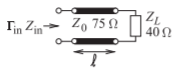
Figure \(\PageIndex{5}\)

Consider the circuit below, a \(60\:\Omega\) lossless line is terminated in a \(40\:\Omega\) load. What is the center of the reflection coefficient locus on the complex plane when it is referenced to \(55\:\Omega\)? [Parallels Example 3.5.2]

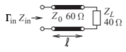
Figure \(\PageIndex{6}\)

3.8.1 Exercises by Section

\(†\)challenging

\(§3.2\: 1, 2, 3†, 4†, 5†, 6†, 7†, 8†, 9†, 10†, 11, 12\)

\(§3.4\: 13, 14, 15, 16, 17, 18, 19, 20, 21, 22, 23, 24, 25, 26, 27, 28, 29, 30, 31, 32, 33, 34, 35, 36, 37†, 38†, 39†, 40†, 41†, 42†\)

\(§3.5\: 43†, 44†\)

3.8.2 Answers to Selected Exercises

\(\frac{\beta}{1-\tau\gamma}(\alpha a_{1}+\gamma a_{2})\)

\(0.940\text{ mW}\)

\(\left[\begin{array}{ll}{-0.2}&{0.8\angle -45^{\circ}}\\{-0.2}&{0.2}\end{array}\right]\)

(d) \(a+\frac{dc^{2}}{1-bd}\)

\(\Gamma_{\text{IN}}=10^{-10}\)

(c) ii & iii
(d) \(8.37-\jmath 49.3\:\Omega\)

\(0.825\angle -50.9^{\circ}\)
\(\approx 250-\jmath 41\:\Omega\)

\(0.0418\)

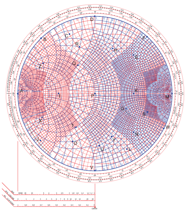
Figure \(\PageIndex{7}\)