
1.9: Fields in Lossy Mediums
- Page ID
- 41010

\( \newcommand{\vecs}[1]{\overset { \scriptstyle \rightharpoonup} {\mathbf{#1}} } \)
\( \newcommand{\vecd}[1]{\overset{-\!-\!\rightharpoonup}{\vphantom{a}\smash {#1}}} \)
\( \newcommand{\id}{\mathrm{id}}\) \( \newcommand{\Span}{\mathrm{span}}\)
( \newcommand{\kernel}{\mathrm{null}\,}\) \( \newcommand{\range}{\mathrm{range}\,}\)
\( \newcommand{\RealPart}{\mathrm{Re}}\) \( \newcommand{\ImaginaryPart}{\mathrm{Im}}\)
\( \newcommand{\Argument}{\mathrm{Arg}}\) \( \newcommand{\norm}[1]{\| #1 \|}\)
\( \newcommand{\inner}[2]{\langle #1, #2 \rangle}\)
\( \newcommand{\Span}{\mathrm{span}}\)
\( \newcommand{\id}{\mathrm{id}}\)
\( \newcommand{\Span}{\mathrm{span}}\)
\( \newcommand{\kernel}{\mathrm{null}\,}\)
\( \newcommand{\range}{\mathrm{range}\,}\)
\( \newcommand{\RealPart}{\mathrm{Re}}\)
\( \newcommand{\ImaginaryPart}{\mathrm{Im}}\)
\( \newcommand{\Argument}{\mathrm{Arg}}\)
\( \newcommand{\norm}[1]{\| #1 \|}\)
\( \newcommand{\inner}[2]{\langle #1, #2 \rangle}\)
\( \newcommand{\Span}{\mathrm{span}}\) \( \newcommand{\AA}{\unicode[.8,0]{x212B}}\)
\( \newcommand{\vectorA}[1]{\vec{#1}} % arrow\)
\( \newcommand{\vectorAt}[1]{\vec{\text{#1}}} % arrow\)
\( \newcommand{\vectorB}[1]{\overset { \scriptstyle \rightharpoonup} {\mathbf{#1}} } \)
\( \newcommand{\vectorC}[1]{\textbf{#1}} \)
\( \newcommand{\vectorD}[1]{\overrightarrow{#1}} \)
\( \newcommand{\vectorDt}[1]{\overrightarrow{\text{#1}}} \)
\( \newcommand{\vectE}[1]{\overset{-\!-\!\rightharpoonup}{\vphantom{a}\smash{\mathbf {#1}}}} \)
\( \newcommand{\vecs}[1]{\overset { \scriptstyle \rightharpoonup} {\mathbf{#1}} } \)
\( \newcommand{\vecd}[1]{\overset{-\!-\!\rightharpoonup}{\vphantom{a}\smash {#1}}} \)
\(\newcommand{\avec}{\mathbf a}\) \(\newcommand{\bvec}{\mathbf b}\) \(\newcommand{\cvec}{\mathbf c}\) \(\newcommand{\dvec}{\mathbf d}\) \(\newcommand{\dtil}{\widetilde{\mathbf d}}\) \(\newcommand{\evec}{\mathbf e}\) \(\newcommand{\fvec}{\mathbf f}\) \(\newcommand{\nvec}{\mathbf n}\) \(\newcommand{\pvec}{\mathbf p}\) \(\newcommand{\qvec}{\mathbf q}\) \(\newcommand{\svec}{\mathbf s}\) \(\newcommand{\tvec}{\mathbf t}\) \(\newcommand{\uvec}{\mathbf u}\) \(\newcommand{\vvec}{\mathbf v}\) \(\newcommand{\wvec}{\mathbf w}\) \(\newcommand{\xvec}{\mathbf x}\) \(\newcommand{\yvec}{\mathbf y}\) \(\newcommand{\zvec}{\mathbf z}\) \(\newcommand{\rvec}{\mathbf r}\) \(\newcommand{\mvec}{\mathbf m}\) \(\newcommand{\zerovec}{\mathbf 0}\) \(\newcommand{\onevec}{\mathbf 1}\) \(\newcommand{\real}{\mathbb R}\) \(\newcommand{\twovec}[2]{\left[\begin{array}{r}#1 \\ #2 \end{array}\right]}\) \(\newcommand{\ctwovec}[2]{\left[\begin{array}{c}#1 \\ #2 \end{array}\right]}\) \(\newcommand{\threevec}[3]{\left[\begin{array}{r}#1 \\ #2 \\ #3 \end{array}\right]}\) \(\newcommand{\cthreevec}[3]{\left[\begin{array}{c}#1 \\ #2 \\ #3 \end{array}\right]}\) \(\newcommand{\fourvec}[4]{\left[\begin{array}{r}#1 \\ #2 \\ #3 \\ #4 \end{array}\right]}\) \(\newcommand{\cfourvec}[4]{\left[\begin{array}{c}#1 \\ #2 \\ #3 \\ #4 \end{array}\right]}\) \(\newcommand{\fivevec}[5]{\left[\begin{array}{r}#1 \\ #2 \\ #3 \\ #4 \\ #5 \\ \end{array}\right]}\) \(\newcommand{\cfivevec}[5]{\left[\begin{array}{c}#1 \\ #2 \\ #3 \\ #4 \\ #5 \\ \end{array}\right]}\) \(\newcommand{\mattwo}[4]{\left[\begin{array}{rr}#1 \amp #2 \\ #3 \amp #4 \\ \end{array}\right]}\) \(\newcommand{\laspan}[1]{\text{Span}\{#1\}}\) \(\newcommand{\bcal}{\cal B}\) \(\newcommand{\ccal}{\cal C}\) \(\newcommand{\scal}{\cal S}\) \(\newcommand{\wcal}{\cal W}\) \(\newcommand{\ecal}{\cal E}\) \(\newcommand{\coords}[2]{\left\{#1\right\}_{#2}}\) \(\newcommand{\gray}[1]{\color{gray}{#1}}\) \(\newcommand{\lgray}[1]{\color{lightgray}{#1}}\) \(\newcommand{\rank}{\operatorname{rank}}\) \(\newcommand{\row}{\text{Row}}\) \(\newcommand{\col}{\text{Col}}\) \(\renewcommand{\row}{\text{Row}}\) \(\newcommand{\nul}{\text{Nul}}\) \(\newcommand{\var}{\text{Var}}\) \(\newcommand{\corr}{\text{corr}}\) \(\newcommand{\len}[1]{\left|#1\right|}\) \(\newcommand{\bbar}{\overline{\bvec}}\) \(\newcommand{\bhat}{\widehat{\bvec}}\) \(\newcommand{\bperp}{\bvec^\perp}\) \(\newcommand{\xhat}{\widehat{\xvec}}\) \(\newcommand{\vhat}{\widehat{\vvec}}\) \(\newcommand{\uhat}{\widehat{\uvec}}\) \(\newcommand{\what}{\widehat{\wvec}}\) \(\newcommand{\Sighat}{\widehat{\Sigma}}\) \(\newcommand{\lt}{<}\) \(\newcommand{\gt}{>}\) \(\newcommand{\amp}{&}\) \(\definecolor{fillinmathshade}{gray}{0.9}\)Lossy mediums result in power loss of EM fields. In RF and microwave systems materials are ideally either perfect conductors or perfect dielectrics. In practice, conductors and dielectrics have finite conductivity and dielectrics have another type of loss called dielectric relaxation loss. Dielectric relaxation loss is due to heating that can result from the movement of charge centers in a material.
1.9.1 Lossy Dielectrics
In a lossy dielectric there can be both current flow and relaxation loss. Current flow results from applied electric field and is described by the conductivity, \(\sigma\), of the material. Relaxation loss results from polarization of the material and the transfer of energy to the lattice of the material as the electric field changes direction. This is also referred to as dielectric damping. The polarization vector describes the additional energy storage capacity of a material (above that of vacuum) in response to an applied electric field. The capacity is described by the electric susceptibility, \(χ_{e}\), in Equation (1.5.20). In phasor form, loss is captured by a complex \(χ_{e}\) or a complex permittivity:
\[\label{eq:1}\varepsilon =\varepsilon'-\jmath\varepsilon''=\varepsilon (1+χ_{e}) \]
Both current and relaxation respond to an applied electric field. In phasor form, Maxwell’s curl equation for a magnetic field, Equation (1.5.32), becomes
\[\begin{align}\nabla\times\overline{H}&=\jmath\omega\overline{D}+\overline{J}=\jmath\omega\varepsilon\overline{E}+\sigma\overline{E}=\jmath\omega(\varepsilon'-\jmath\varepsilon'')\overline{E}+\sigma\overline{E}\nonumber \\&=\jmath\omega\varepsilon'\overline{E}+(\sigma +\omega\varepsilon'')\overline{E}\nonumber \\ \label{eq:2}&=\jmath\omega\left(\varepsilon'-\jmath\varepsilon''-\jmath\frac{\sigma}{\omega}\right)\overline{E}\end{align} \]
In the above, \(\omega\varepsilon'\) describes the ability to store electric energy, \(\omega\varepsilon''\) describes dielectric damping loss, and \(\sigma\) describes conductivity loss. At a single frequency, damping and conductivity losses are indistinguishable and so the term \((\omega\varepsilon''+\sigma)\) is taken as the effective conductivity. The effective (complex) relative permittivity is
\[\label{eq:3}\varepsilon_{e}=\left(\varepsilon'-\jmath\varepsilon''-\jmath\frac{\sigma}{\omega}\right)\frac{1}{\varepsilon_{0}} \]
Another quantity that describes loss is the loss tangent, \(\tan\delta\), which is the ratio of power lost to energy stored:
\[\label{eq:4}\tan\delta =\frac{\omega\varepsilon''+\sigma}{\omega\varepsilon'} \]
For many dielectric materials used with EM structures, \(\tan\delta\) is approximately independent of frequency up to \(100\)s of gigahertz, so it is commonly used to characterize the dielectric loss of a material. Most exceptions are semiconductors such as silicon which can have appreciable conductive loss. The frequency independence of \(\tan\delta\) indicates that conductivity loss is negligible.
Consider a plane EM wave propagating in a medium with permittivity \(\varepsilon\) and permeability \(\mu\). The complex permittivity measured at two frequencies is experimentally characterized by the relative permittivity \((\varepsilon /\varepsilon_{0})\) of the real, \(\Re\{\varepsilon /\varepsilon_{0}\}\), and imaginary, \(ℑ \{\varepsilon /\varepsilon_{0}\}\), parts as follows:
Measured relative permittivity:
| Frequency | Real Part | Imaginary Part |
|---|---|---|
| \(1\text{ GHz}\) | \(1.9\) | \(-0.0490\) |
| \(2\text{ GHz}\) | \(1.9\) | \(-0.0314\) |
Table \(\PageIndex{2}\)
Measured relative permeability:
| Frequency | Real Part | Imaginary Part |
|---|---|---|
| \(1\text{ GHz}\) | \(1.9\) | \(-0.001\) |
| \(2\text{ GHz}\) | \(1.9\) | \(-0.001\) |
Table \(\PageIndex{3}\)
Since there is an imaginary part of the dielectric constant, there could be loss due to either dielectric damping or finite material conductivity, or both. When characterizing materials, it is only possible to distinguish the contribution to the measured imaginary part of the permittivity by considering the experimentally derived imaginary permittivity at two different frequencies.
- Determine the dielectric loss tangent at \(1\text{ GHz}\).
- Determine the relative dielectric damping factor at \(1\text{ GHz}\) (the part of the permittivity due to dielectric damping).
- What is the conductivity of the dielectric?
- What is the magnetic conductivity of the medium?
Solution
- At \(1\text{ GHz}\), \(\varepsilon =\varepsilon_{r}\varepsilon_{0}\), and the measured relative permittivity is
\[\label{eq:5}\varepsilon_{r}=1.9-\jmath 0.049=\varepsilon_{r, e}'-\jmath\varepsilon_{r, r}'' \]
where \(\varepsilon_{r, e}'\) and \(\varepsilon_{r, e}''\) are the effective (measured) values of \(\varepsilon_{r}'\) and \(\varepsilon_{r}''\) obtained from measurement. Now \(\varepsilon_{e}'=\varepsilon'\), but the imaginary permittivity includes the effect of dielectric conductivity, \(\sigma\), as well as of dielectric damping, which is described by \(\varepsilon''\) alone. That is,
\[\label{eq:6}\varepsilon_{e}'' =\varepsilon'' +\frac{\sigma}{\omega}\cdot\varepsilon_{r} =\varepsilon_{r, e}'' = 0.0490\quad\text{ and}\quad \tan\delta = 0.0490/1.9=0.0258 \] - The imaginary relative permittivity is found by noting that \(\varepsilon_{r, e}'' =\varepsilon_{r}'' +\sigma/\omega\) and \(\omega\varepsilon_{r}'' +\sigma =\omega\varepsilon_{r,e}''\). Let \(\omega_{1} = 2π\) (\(1\text{ GHz}\)). Then
\[\begin{aligned}\omega_{2}&=2\omega_{1}\nonumber \\ \omega_{1}\varepsilon_{r, e}''(1\text{ GHz})&=\omega_{1}\varepsilon_{r}''+\sigma =\omega_{1}\cdot 0.0490& (\text{A})\nonumber \\ \omega_{2}\varepsilon_{r, e}''(2\text{ GHz})&=\omega_{2}\varepsilon_{r}''+\sigma =\omega_{2}\cdot 0.0314\nonumber \\ 2\omega_{1}\varepsilon_{e}''+\sigma&=2\omega_{1}(0.0314)& (\text{B})\nonumber \\ (\text{B})-(\text{A})\to\omega_{1}\varepsilon_{r}''&=\omega_{1}[0.0628-0.0490]\nonumber \\ \varepsilon_{r}''&=0.0138\text{ (at all frequencies)}\nonumber \end{aligned} \nonumber \] - Recall that \(\varepsilon_{r,e}'' =\varepsilon_{r}''+\sigma/\omega\)
At \(1\text{ GHz}\), \(\omega = 2\pi\times 10^{9}\), \(\varepsilon_{r,e}'' = 0.0490\), \(\varepsilon_{r}'' = 0.0138\), so
\[\sigma =\omega\left(\varepsilon_{r, e}''-\varepsilon_{r}''\right) = 2\cdot\pi\cdot 10^{9} (0.0490 − 0.0138) = 0.221\cdot 10^{9}\text{ S/m} = 221\text{ MS/m}\nonumber \] - Magnetic conductivity is nonexistent, thus magnetic conductivity is zero.
1.9.2 Lossy Conductors
Perfect conductors would have infinite conductivity, but since the conductivity of real conductors is finite, EM fields penetrate into the interior of a conductor. Still the energy stored in the current is much greater than the (dielectric) electric energy storage capability, \(\sigma ≫ \omega\varepsilon'\), and the losses from conductivity are much higher than dielectric loss, \(\sigma ≫ \omega\varepsilon''\), so that the effective relative permittivity from Equation \(\eqref{eq:3}\) is
\[\label{eq:7}\varepsilon_{e}=\left(\varepsilon'-\jmath\varepsilon''-\jmath\frac{\sigma}{\omega}\right)\frac{1}{\varepsilon_{0}}\approx\left(-\jmath\frac{\sigma}{\omega}\right)\frac{1}{\varepsilon_{0}}\approx\left(\frac{\sigma}{\jmath\omega}\right)\frac{1}{\varepsilon{0}} \]
For most conductors the permeability is \(\mu_{0}\) and the working permittivity is
\[\label{eq:8}\varepsilon =\varepsilon_{e}\varepsilon_{0}=\frac{\sigma}{\jmath\omega} \]
The propagation constant of the field in a conductor is
\[\label{eq:9}\gamma =\alpha+\jmath\beta\approx\jmath\omega\sqrt{\mu\varepsilon}\approx\jmath\omega\sqrt{\mu}\sqrt{\frac{\sigma}{\jmath\omega}}\approx (1+\jmath)\sqrt{\frac{\omega\mu\sigma}{2}} \]
So \(\alpha =\sqrt{\omega\mu\sigma /2}\). The EM field in the conductor reduces in amplitude as \(e^{−\alpha x}\) after a distance \(x\). Thus the field reduces to \(1/e\) of its value after a distance called the skin depth, \(\delta_{s}\):
\[\label{eq:10}\delta_{s}=\sqrt{\frac{2}{\omega\mu\sigma}} \]
If the amplitude of the electric field at the surface of a conductor is \(A(0)\), after a distance \(\delta_{s}\) the amplitude of the electric field will have the amplitude
\[\begin{align}A(\delta_{s})&=e^{-\alpha x}=e^{-\left(\sqrt{\omega\mu\sigma/2}\sqrt{2/\omega\mu\sigma}\right)}\nonumber \\ \label{eq:11}&=e^{-1}\end{align} \]
Table \(\PageIndex{4}\) lists the skin depth and phase velocities of conductors commonly used in microwave circuits. The resistivity values here are those of a single crystal. The phase velocity, \(v_{p}\), is calculated from the propagation constant \(\beta\). From Equation \(\eqref{eq:9}\), \(\beta=\sqrt{\omega\mu\sigma /2}\).
\[\label{eq:12}\text{Now }v_{p}=\omega /\beta\text{, so that}\quad v_{p}=\frac{\omega}{\beta}=\frac{\omega\sqrt{2}}{\sqrt{\omega\mu\sigma}}=\sqrt{\frac{2\omega}{\mu\sigma}} \]
This can be simplified further if the relative permeability of the material is \(1\), as then \(\mu = \mu_{0} = 4\pi 10^{−7}\text{ H/m}\). If SI units are used for \(f\) and \(\sigma\):
\[\label{eq:13}v_{p}=\sqrt{\frac{2\omega}{\mu_{0}\sigma}}=\sqrt{\frac{4\pi f}{4\pi 10^{-7}\sigma}}=\sqrt{\frac{10^{7}f}{\sigma}} \]
From Table \(\PageIndex{4}\) note that the skin depth at gigahertz frequencies is close to the thickness of microstrip lines which are often only a few microns thick. Also the speed of an EM wave in a conductor is very slow. The speed of EM in copper (ideal), for example, is \(0.004\%\) of the speed of light in a vacuum.
| Material | Electrical conductivity, \(\sigma\) \((\text{MS.m}^{-1})\) | Skin depth, \(\delta\) at \(1\text{ GHz}\) \((\mu\text{m})\) | Phase velocity, \(v_{p}\) at \(1\text{ GHz}\) \((\text{km/s})\) |
|---|---|---|---|
| \(1\text{ GHz}\) | |||
| Aluminum (crystal) | \(37.7\) | \(2.59\) | \(16.3\) |
| Aluminum (\(2\times\) resistivity) | \(18.9\) | \(3.66\) | \(23.0\) |
| Copper (single crystal) | \(59.6\) | \(2.06\) | \(13.0\) |
| Copper (\(2\times\) resistivity) | \(29.8\) | \(2.92\) | \(18.3\) |
| Gold (single crystal) | \(45.2\) | \(2.37\) | \(14.9\) |
| Gold (\(2\times\) resistivity) | \(22.6\) | \(3.35\) | \(21.0\) |
| Silver (single crystal) | \(63.0\) | \(2.01\) | \(12.6\) |
| Silver (\(2\times\) resistivity) | \(31.5\) | \(2.84\) | \(17.8\) |
| Titanium (single crystal) | \(0.238\) | \(32.6\) | \(200\) |
| Titanium (\(2\times\) resistivity) | \(0.119\) | \(46.1\) | \(290\) |
Table \(\PageIndex{4}\): Skin depth and effective phase velocity at \(1\text{ GHz}\) of several conductors commonly used in microwave circuits.
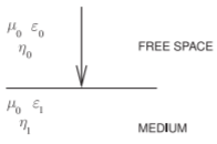
Figure \(\PageIndex{1}\): Two regions used in Example \(\PageIndex{2}\).
This example provides a review of basic EM theory. In Figure \(\PageIndex{1}\), a plane wave in free space is normally incident on a lossless medium occupying a half space with a dielectric constant of \(16\). Calculate the electric field reflection coefficient at the interface referred to the medium.
Solution
Since it is not explicitly stated, assume \(\mu_{1} =\mu_{0}\). (This should be done in general since \(\mu_{0}\) is the default value for \(\mu\), as most materials have unity relative permeability.) The characteristic impedance of a medium is \(\eta = \sqrt{mu/\varepsilon}\). Now \(\eta\) is used for characteristic impedance (also called wave impedance) of a TEM propagating wave in a medium. It is used instead of \(Z_{0}\), which is generally reserved for the characteristic impedance of transmission lines. The electric field reflection coefficient is
\[\Gamma^{E}=\frac{\eta_{1}-\eta_{0}}{\eta_{1}+\eta_{0}}=\frac{\eta_{1}/\eta_{0}-1}{\eta_{1}/\eta_{0}+1}\nonumber \]
\[\frac{\eta_{1}}{\eta_{0}}=\sqrt{\frac{\mu_{0}}{\varepsilon_{1}}}\cdot\sqrt{\frac{\varepsilon_{0}}{\mu_{0}}}=\sqrt{\frac{\varepsilon_{0}}{\varepsilon_{1}}}=\sqrt{\frac{1}{16}}=\frac{1}{4}\nonumber \]
so
\[\Gamma^{E}=\frac{1/4-1}{1/4+1}=\frac{1-4}{1+4}=-\frac{3}{5}=-0.6\nonumber \]
This example provides an intuitive way of solving an EM problem. A plane wave in free space is normally incident on a lossless medium occupying a half space with a dielectric constant of \(16\). What is the magnetic field reflection coefficient?
Solution
There are two ways to answer this question. An intuitive approach will be used first.
Intuitively \(|\Gamma^{H}|=|\Gamma^{E}|\),
With \(\overline{\mathcal{E}}\) and \(\overline{\mathcal{H}}\) being vectors, the Poynting vector \(\overline{\mathcal{E}}\times\overline{\mathcal{H}}\) points in the direction of propagation for a plane wave, since the reflected wave is in the opposite direction to the incident wave, thus
\[\text{sign}\left(\Gamma^{H}\right)=-\text{sign}\left(\Gamma^{E}\right)\nonumber \]
Therefore \(\Gamma^{H} = −\Gamma^{E} = +0.6\). (\(\Gamma^{E}\) was calculated in Example \(\PageIndex{2}\).)
Now the second approach. The formula for the magnetic field reflection coefficient is
\[\Gamma_{H}=\frac{\eta_{1}-\eta_{2}}{\eta_{1}+\eta_{2}}=\frac{1-\eta_{2}/\eta_{1}}{1+\eta_{2}/\eta_{1}}=\frac{1-1/4}{1+1/4}=\frac{3}{5}=0.6\nonumber \]
A \(4\text{ GHz}\) time-varying EM field is traveling in the \(+z\) direction in Region 1 and is normally incident on another material in Region 2. The boundary between the two regions is in the \(z = 0\) plane. The permittivity of Region 1 is \(\varepsilon_{1} =\varepsilon_{0}\) and that of Region 2 is \(\varepsilon_{2} = (4 −\jmath 0.4)\varepsilon_{0}\). For both regions, \(\mu_{1} =\mu_{2} =\mu_{0}\). The phasor of the forward-traveling electric field (i.e., the incident field) is \(\mathbf{E}^{+} = 100\hat{y}\), and the phase is normalized with respect to \(z = 0\).
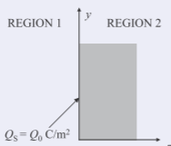
Figure \(\PageIndex{2}\)
What are the wave impedance and propagation constant of Region 2?
Solution
The wave impedance is
\[\begin{align}\eta&=\sqrt{\frac{\mu}{\varepsilon}}=\sqrt{\frac{\mu_{0}}{\varepsilon_{0}}}\sqrt{\frac{\mu_{r}}{\varepsilon_{r}}}=\eta_{0}\sqrt{\frac{\mu_{r}}{\varepsilon_{r}}}=377\sqrt{\frac{1}{(4-\jmath 0.4)}\Omega}\nonumber \\ \label{eq:14}&=187.8+\jmath 9.4\:\Omega\end{align} \]
The propagation constant is
\[\begin{align}\gamma&=\jmath\omega\sqrt{\mu\varepsilon}=\jmath\omega\sqrt{\mu_{0}\varepsilon_{0}}\sqrt{\mu_{r}\varepsilon_{r}}\nonumber \\ \label{eq:15}&=\jmath 4\cdot 2\pi\cdot 10^{9}\cdot\sqrt{4\pi\cdot 10^{-7}\cdot 8.854\cdot 10^{-12}}\sqrt{4-\jmath 0.4}=(8.4+\jmath 167.9)\text{m}^{-1}\end{align} \]