
3.7: Stripline
- Page ID
- 41033

\( \newcommand{\vecs}[1]{\overset { \scriptstyle \rightharpoonup} {\mathbf{#1}} } \)
\( \newcommand{\vecd}[1]{\overset{-\!-\!\rightharpoonup}{\vphantom{a}\smash {#1}}} \)
\( \newcommand{\dsum}{\displaystyle\sum\limits} \)
\( \newcommand{\dint}{\displaystyle\int\limits} \)
\( \newcommand{\dlim}{\displaystyle\lim\limits} \)
\( \newcommand{\id}{\mathrm{id}}\) \( \newcommand{\Span}{\mathrm{span}}\)
( \newcommand{\kernel}{\mathrm{null}\,}\) \( \newcommand{\range}{\mathrm{range}\,}\)
\( \newcommand{\RealPart}{\mathrm{Re}}\) \( \newcommand{\ImaginaryPart}{\mathrm{Im}}\)
\( \newcommand{\Argument}{\mathrm{Arg}}\) \( \newcommand{\norm}[1]{\| #1 \|}\)
\( \newcommand{\inner}[2]{\langle #1, #2 \rangle}\)
\( \newcommand{\Span}{\mathrm{span}}\)
\( \newcommand{\id}{\mathrm{id}}\)
\( \newcommand{\Span}{\mathrm{span}}\)
\( \newcommand{\kernel}{\mathrm{null}\,}\)
\( \newcommand{\range}{\mathrm{range}\,}\)
\( \newcommand{\RealPart}{\mathrm{Re}}\)
\( \newcommand{\ImaginaryPart}{\mathrm{Im}}\)
\( \newcommand{\Argument}{\mathrm{Arg}}\)
\( \newcommand{\norm}[1]{\| #1 \|}\)
\( \newcommand{\inner}[2]{\langle #1, #2 \rangle}\)
\( \newcommand{\Span}{\mathrm{span}}\) \( \newcommand{\AA}{\unicode[.8,0]{x212B}}\)
\( \newcommand{\vectorA}[1]{\vec{#1}} % arrow\)
\( \newcommand{\vectorAt}[1]{\vec{\text{#1}}} % arrow\)
\( \newcommand{\vectorB}[1]{\overset { \scriptstyle \rightharpoonup} {\mathbf{#1}} } \)
\( \newcommand{\vectorC}[1]{\textbf{#1}} \)
\( \newcommand{\vectorD}[1]{\overrightarrow{#1}} \)
\( \newcommand{\vectorDt}[1]{\overrightarrow{\text{#1}}} \)
\( \newcommand{\vectE}[1]{\overset{-\!-\!\rightharpoonup}{\vphantom{a}\smash{\mathbf {#1}}}} \)
\( \newcommand{\vecs}[1]{\overset { \scriptstyle \rightharpoonup} {\mathbf{#1}} } \)
\( \newcommand{\vecd}[1]{\overset{-\!-\!\rightharpoonup}{\vphantom{a}\smash {#1}}} \)
\(\newcommand{\avec}{\mathbf a}\) \(\newcommand{\bvec}{\mathbf b}\) \(\newcommand{\cvec}{\mathbf c}\) \(\newcommand{\dvec}{\mathbf d}\) \(\newcommand{\dtil}{\widetilde{\mathbf d}}\) \(\newcommand{\evec}{\mathbf e}\) \(\newcommand{\fvec}{\mathbf f}\) \(\newcommand{\nvec}{\mathbf n}\) \(\newcommand{\pvec}{\mathbf p}\) \(\newcommand{\qvec}{\mathbf q}\) \(\newcommand{\svec}{\mathbf s}\) \(\newcommand{\tvec}{\mathbf t}\) \(\newcommand{\uvec}{\mathbf u}\) \(\newcommand{\vvec}{\mathbf v}\) \(\newcommand{\wvec}{\mathbf w}\) \(\newcommand{\xvec}{\mathbf x}\) \(\newcommand{\yvec}{\mathbf y}\) \(\newcommand{\zvec}{\mathbf z}\) \(\newcommand{\rvec}{\mathbf r}\) \(\newcommand{\mvec}{\mathbf m}\) \(\newcommand{\zerovec}{\mathbf 0}\) \(\newcommand{\onevec}{\mathbf 1}\) \(\newcommand{\real}{\mathbb R}\) \(\newcommand{\twovec}[2]{\left[\begin{array}{r}#1 \\ #2 \end{array}\right]}\) \(\newcommand{\ctwovec}[2]{\left[\begin{array}{c}#1 \\ #2 \end{array}\right]}\) \(\newcommand{\threevec}[3]{\left[\begin{array}{r}#1 \\ #2 \\ #3 \end{array}\right]}\) \(\newcommand{\cthreevec}[3]{\left[\begin{array}{c}#1 \\ #2 \\ #3 \end{array}\right]}\) \(\newcommand{\fourvec}[4]{\left[\begin{array}{r}#1 \\ #2 \\ #3 \\ #4 \end{array}\right]}\) \(\newcommand{\cfourvec}[4]{\left[\begin{array}{c}#1 \\ #2 \\ #3 \\ #4 \end{array}\right]}\) \(\newcommand{\fivevec}[5]{\left[\begin{array}{r}#1 \\ #2 \\ #3 \\ #4 \\ #5 \\ \end{array}\right]}\) \(\newcommand{\cfivevec}[5]{\left[\begin{array}{c}#1 \\ #2 \\ #3 \\ #4 \\ #5 \\ \end{array}\right]}\) \(\newcommand{\mattwo}[4]{\left[\begin{array}{rr}#1 \amp #2 \\ #3 \amp #4 \\ \end{array}\right]}\) \(\newcommand{\laspan}[1]{\text{Span}\{#1\}}\) \(\newcommand{\bcal}{\cal B}\) \(\newcommand{\ccal}{\cal C}\) \(\newcommand{\scal}{\cal S}\) \(\newcommand{\wcal}{\cal W}\) \(\newcommand{\ecal}{\cal E}\) \(\newcommand{\coords}[2]{\left\{#1\right\}_{#2}}\) \(\newcommand{\gray}[1]{\color{gray}{#1}}\) \(\newcommand{\lgray}[1]{\color{lightgray}{#1}}\) \(\newcommand{\rank}{\operatorname{rank}}\) \(\newcommand{\row}{\text{Row}}\) \(\newcommand{\col}{\text{Col}}\) \(\renewcommand{\row}{\text{Row}}\) \(\newcommand{\nul}{\text{Nul}}\) \(\newcommand{\var}{\text{Var}}\) \(\newcommand{\corr}{\text{corr}}\) \(\newcommand{\len}[1]{\left|#1\right|}\) \(\newcommand{\bbar}{\overline{\bvec}}\) \(\newcommand{\bhat}{\widehat{\bvec}}\) \(\newcommand{\bperp}{\bvec^\perp}\) \(\newcommand{\xhat}{\widehat{\xvec}}\) \(\newcommand{\vhat}{\widehat{\vvec}}\) \(\newcommand{\uhat}{\widehat{\uvec}}\) \(\newcommand{\what}{\widehat{\wvec}}\) \(\newcommand{\Sighat}{\widehat{\Sigma}}\) \(\newcommand{\lt}{<}\) \(\newcommand{\gt}{>}\) \(\newcommand{\amp}{&}\) \(\definecolor{fillinmathshade}{gray}{0.9}\)A symmetrical stripline is shown in Figure \(\PageIndex{1}\)(a). A stripline resembles a microstrip line and comprises a center conductor pattern symmetrically embedded completely within a dielectric, the top and bottom layers of which are conducting ground planes. The strip of width \(w\) is considered to have a thickness \(t\) that is very small so that the strip is a distance \(h\) from each of the ground planes and the ground planes are separated by \(b = 2h\)D. The strip is completely surrounded by the dielectric and so this is a homogeneous medium and there is no need to introduce an effective permittivity.
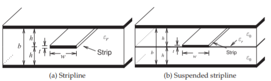
Figure \(\PageIndex{1}\): Stripline transmission lines. In the suspended stripline the strip is supported by a membrane.
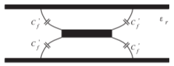
Figure \(\PageIndex{2}\): Fringe capacitance at the corners of the strip in a stripline transmission lines.
3.7.1 Characteristic Impedance of a Stripline
Finite Thickness
The characteristic impedance of a stripline is [25, 26]
\[\label{eq:1}Z_{0}=\left[\frac{30\pi}{\sqrt{\varepsilon_{r}}}\right]\frac{(1-t/b)}{(w_{\text{eff}}/b)+C_{f}} \]
where the effective width of the strip, \(w_{\text{eff}}\), is obtained from
\[\label{eq:2}\frac{w_{\text{eff}}}{b}=\left\{\begin{array}{ll}{\frac{w}{b}-\left[\frac{(0.35-w/b)^{2}}{(1+12t/b)}\right]}&{\frac{w}{b}<0.35}\\{\frac{w}{b}}&{\frac{w}{b}\geq 0.35}\end{array}\right. \]
and
\[\label{eq:3}C_{f}=\frac{2}{\pi}\ln\left[\frac{1}{1-(t/b)}+1\right]-\frac{t}{\pi b}\ln\left\{\frac{1}{[1-(t/b)]^{2}}-1\right\} \]
\(C_{f}\) accounts for the fringing capacitance at the edges of the strip and incorporates the effect of the strip thickness for \(t ≪ b\). The fringing capacitance per unit length (e.g., \(\text{F/m}\)) at each corner of the strip is
\[\label{eq:4}C_{f}'=\frac{\epsilon_{0}\varepsilon_{r}C_{f}}{1-t/b} \]
and is shown in Figure \(\PageIndex{2}\). The accuracy of these formulas is better than \(1\%\) for \(W/(b − t) > 0.05\) and \(t/b < 0.025\).
Zero Thickness
If the strip has zero thickness, the characteristic impedance of stripline is
\[\label{eq:5}Z_{0}=\left[\frac{30\pi}{\sqrt{\varepsilon_{r}}}\right]\frac{1}{(w_{\text{eff}}/b)+2\ln 2/\pi}=\frac{94.25}{\sqrt{\varepsilon_{r}}}\frac{1}{(w_{\text{eff}}/b)+0.441} \]
where the effective width of the strip, \(w_{\text{eff}}\), is obtained from
\[\label{eq:6}\frac{w_{\text{eff}}}{b}=\left\{\begin{array}{ll}{\frac{w}{b}-\left(0.35-\frac{w}{b}\right)^{2}}&{\frac{w}{b}<0.35}\\{\frac{w}{b}}&{\frac{w}{b}\geq 0.35}\end{array}\right. \]
The fringing capacitance per unit length at each corner of the strip is
\[\label{eq:7}C_{f}'=\frac{\epsilon_{0}\varepsilon_{r}2\ln2}{\pi}=0.441\epsilon_{0}\varepsilon_{r} \]
A stripline supports a purely TEM mode and there is no dielectric dispersion due to an effective permittivity change with frequency. Losses in a stripline are due to dielectric, conductor, and radiative losses. Radiative losses are confined to energy lost to excitation of the parallel plate waveguide mode, but this can be suppressed by shorting the ground planes together at regular intervals (say every tenth of a wavelength).
Formulas have also been developed for the characteristic impedance of asymmetrical stripline, that is, when the strip is not centered between the ground planes [27].
A thin strip of a symmetrical stripline has a width of \(0.5\text{ mm}\), is embedded in a dielectric of relative permittivity \(5.6\), and is between ground planes separated by \(1\text{ mm}\). What is the characteristic impedance of the stripline?
Solution
The structure is shown in Figure \(\PageIndex{1}\)(a) with \(w = 0.5\text{ mm}\) and \(b = 1\text{ mm}\). Since the strip is thin, consider that \(t = 0\). So from Equations \(\eqref{eq:2}\) and \(\eqref{eq:3}\)
\[\label{eq:8}\frac{w_{\text{eff}}}{b}=0.5\quad\text{and}\quad C_{f}=0.441 \]
and so
\[\label{eq:9}Z_{0}=\frac{94.25}{\sqrt{5.6}}\frac{1}{(0.5+0.441)}=42.77\:\Omega \]
3.7.2 Attenuation on a Stripline
For a low-loss stripline with radiation loss suppressed by vias between the ground planes, the attenuation, \(\alpha\), comprises two parts, the conductive attenuation, \(\alpha_{c}\), and the dielectric attenuation, \(\alpha_{d}\), so that \(\alpha=\alpha_{c}+\alpha_{d}\). From Equation (2.5.15)
\[\label{eq:10}\alpha_{c}=\frac{R}{2Z_{0}} \]
where \(R\) is the resistance per unit length of the line. \(R\) is the sum of the strip and ground resistances. At low frequencies the resistance of the strip is
\[\label{eq:11}R_{\text{strip}}=R_{s}/w \]
where \(R_{s}\) is the sheet resistance of the strip and \(w\) is the width of the strip. The treatment for the ground resistance is similar to that described in Section 3.5.5 for microstrip. At low microwave frequencies
\[\label{eq:12}R_{\text{ground}}=\frac{1}{2}\frac{R_{sg}}{w}\frac{w/h}{w/h+5.8+0.03h/w},\quad\text{for }0.1\leq w/h\leq 10 \]
where the sheet resistance of the ground plane is \(R_{sg}\). The factor of onehalf arises because there are two grounds and the resistance from each is in parallel. The effect of the ground on the line resistance is small. Both \(R_{\text{strip}}\) and \(R_{\text{ground}}\) will increase at higher frequencies as the charges rearrange at much higher frequencies. This will be considered in the next chapter.
The formula for the dielectric attenuation comes from Equation (3.5.26). The general formula for the attenuation constant due to dielectric loss is, for a low-loss TEM line,
\[\label{eq:13}\alpha_{d}=\frac{\omega}{c}(\tan\delta)\frac{\varepsilon_{r}(\varepsilon_{e}-1)}{2\sqrt{\varepsilon_{e}}(\varepsilon_{r}-1)}\text{ Np/m} \]
Since the effective permittivity of a stripline is just the relative permittivity of the substrate, \(\varepsilon_{e} =\varepsilon_{r}\), then Equation \(\eqref{eq:13}\) reduces to
\[\label{eq:14}\alpha_{d}=\frac{\omega}{2c}(\tan\delta)\sqrt{\varepsilon_{r}}\text{ Np/m}=\frac{1}{2}\omega\sqrt{\mu_{0}\varepsilon_{e}\varepsilon_{r}}(\tan\delta)\text{ Np/m} \]
(Note that here \(\omega\) is the radian frequency and not the width \(w\).)
The suspended stripline structure shown in Figure \(\PageIndex{1}\)(b) has minimal dielectric and hence minimal dielectric loss. Resonators built using a suspended stripline have a high \(Q\) and this structure can be used to realize high-performance filters.
What is the attenuation of a symmetrical stripline at \(1\text{ GHz}\) with \(w = h = 0.5\text{ mm}\), a \(t = 4\:\mu\text{m}\)-thick strip, silver metallization, and an FR-4 substrate. The ground planes are \(4\:\mu\text{m}\) thick. Assume that high frequency effects on line resistance can be ignored.
Solution
The strip is very thin and the results of Example \(\PageIndex{1}\) can be used so \(Z_{0} = 42.77\:\Omega\). The resistivity of silver is \(\rho_{\text{Ag}} = 14.87\text{ n}\Omega\cdot\text{m}\) and so the sheet resistivity of the strip, \(R_{s} = \rho_{\text{Ag}}/t = (14.87\text{ n}\Omega\cdot\text{m})/(4\:\mu\text{m})=3.968\text{ m}\Omega\). From Equation \(\eqref{eq:11}\) the resistance of the strip is \(R_{\text{strip}} = R_{s}/w = (3.968\text{ m}\Omega)/(1\text{ mm})=3.968\:\Omega\text{/m}\). The sheet resistance of the grounds is the same as the strip so \(R_{sg} = 3.968\text{ m}\Omega\). From Equation \(\eqref{eq:12}\) the resistance of the grounds is
\[\begin{align} R_{\text{ground}}&=\frac{1}{2}\frac{R_{\text{sg}}}{w}\frac{w/h}{w/h+5.8+0.03h/w} \nonumber \\ \label{eq:15} &=\frac{1}{2}\frac{(3.968\text{ m}\Omega )}{(1\text{ mm})}\frac{1}{1+5.8+0.03}=\frac{3.968\:\Omega\text{/m}}{6.83}=0.581\:\Omega\text{/m}\end{align} \]
so that the total line resistance \(R = R_{\text{strip}} + R_{\text{ground}} = 4.549\:\Omega\text{/m}\). Thus the attenuation due to conductor loss is \(\alpha_{c} = R/(2Z_{0})=0.1064\text{ Np/m} = 0.924\text{ dB/m}\). FR-4 has negligible conductivity and loss in the dielectric is due to dielectric relaxation. FR-4 has a loss tangent at \(1\text{ GHz}\) of \(0.01\) and a relative dielectric constant of \(4.3\). From Equation \(\eqref{eq:14}\)
\[\label{eq:16}\alpha_{d}=\frac{1}{2}\omega\sqrt{\mu_{0}\varepsilon_{0}\varepsilon_{r}}(\tan\delta)\text{ Np/m}=0.2172\text{ Np/m}=1.886\text{ dB/m} \]
The total attenuation \(\alpha =\alpha_{c}+\alpha_{d} = (0.924 + 1.886)\text{ dB/m} = 2.810\text{ dB/m}\).
3.7.3 Design Formulas for a Stripline
The synthesis of a symmetrical stripline with a substrate having a relative permittivity \(\varepsilon_{r}\) and thickness \(b\) requires determination of the width of the strip for a particular characteristic impedance [25]. The width \(w\) is obtained from
\[\label{eq:17}\frac{w}{b}=\left\{\begin{array}{ll}{x}&{\text{for }Z_{0}\leq 120/\sqrt{\varepsilon_{r}}\:\Omega}\\{0.85-\sqrt{0.6-x}}&{\text{for }Z_{0}>120/\sqrt{\varepsilon_{r}}\:\Omega}\end{array}\right. \]
where
\[\label{eq:18}x=\frac{30\pi}{\sqrt{\varepsilon_{r}}Z_{0}}-\frac{2\ln2}{\pi}=\frac{94.25}{\sqrt{\varepsilon_{r}}Z_{0}}-0.441 \]