2.21: Exercises

1. The characteristic function of a doubly terminated network is \(K(s) = s^{2}\).
   1. What is the magnitude-squared transmission coefficient \((|T (s)|^{2})\)?
   2. What is the magnitude-squared reflection coefficient \((|\Gamma (s)|^{2})\)?
   3. What is transmission coefficient \(T(s)\) for a circuit that can be realized using positive \(R,\: L,\) and \(C\) elements)?
2. The characteristic function of a doubly terminated network is \(K(s) = s^{4}\). What is the magnitude-squared transmission coefficient \((|\Gamma (s)|^{2})\)?
3. Consider the design of a fourth-order lowpass Butterworth filter. [This problem follows the development in Section 2.4.]
   1. What is the magnitude-squared characteristic polynomial, \(|K(s)|^{2}\), of the Butterworth filter?
   2. What is the magnitude-squared transmission coefficient (or transfer function)?
   3. What is the magnitude-squared reflection coefficient function?
   4. Derive the reflection coefficient function (i.e., \(\Gamma (s)\)). Write down the reflection coefficient in factorized form using up to second-order factors.
   5. What are the roots of the numerator polynomial of the reflection coefficient function?
   6. What are the roots of the denominator polynomial of the reflection coefficient function?
   7. Identify the conjugate pole pairs in the factorized reflection coefficient.
   8. Plot the poles and zeros of the reflection coefficient on the complex \(s\) plane.
4. Derive the reflection coefficient poles of a second-order Butterworth filter and write out the reflection coefficient with nominator and denominator polynomials, that is not in factorized form. [Parallels Example 2.4.1]
5. Derive the reflection coefficient poles and zeros of a fourth-order Chebyshev filter with a ripple factor, \(\varepsilon\), of \(0.1\).
6. Synthesize the impedance function
   \[Z_{x}=\frac{s^{3}+s^{2}+2s+1}{s^{2}+s+1}\nonumber \]
   That is, develop the \(RLC\) circuit that realizes \(Z_{x}\). [Parallels Example 2.6.1]
7. Synthesize the impedance function
   \[Z_{w}=\frac{4s^{2}+2s+1}{8s^{3}+8s^{2}+2s+1}\nonumber \]
   That is, develop the \(RLC\) circuit that realizes \(Z_{w}\). [Parallels Example 2.6.2]
8. Synthesize the impedance function
   \[Z_{x}=\frac{4s^{2}+2s+1}{4s^{2}+1}\nonumber \]
   That is, develop the \(RLC\) circuit that realizes \(Z_{x}\). [Parallels Example 2.6.1. You may also want to consult Figure 2.6.2.]
9. Synthesize the impedance function
   \[Z_{x}=\frac{4s^{4}+2s^{3}+5s^{2}+2s+1}{4s^{4}+4s^{3}+7s^{2}+s+1}\nonumber \]
   That is, develop the \(RLC\) circuit that realizes \(Z_{x}\). [Parallels Example 2.6.1. You may also want to consult Figure 2.6.2.]
10. Develop the lowpass prototype of a fifth-order Butterworth lowpass filter. There may be more than one solution. That is, draw the circuit of the lowpass filter prototype with element values.
11. Develop the lowpass prototype of a fifth-order Chebyshev lowpass filter with \(1\text{ dB}\) ripple and \(1\text{ rad/s}\) corner frequency.
12. Develop the lowpass prototype of a ninth-order Chebyshev lowpass filter with \(0.01\text{ dB}\) ripple and \(1\text{ rad/s}\) corner frequency.
13. A \(0.04\text{ S}\) admittance inverter is to be implemented in microstrip using a single length of transmission line. The effective permittivity of the line is \(9\) and the design center frequency is \(10\text{ GHz}\).
    1. What is the characteristic impedance of the transmission line?
    2. What is the wavelength in millimeters at the design center frequency in free space?
    3. What is the wavelength in millimeters at the design center frequency in microstrip?
    4. What is electrical length of the microstrip transmission line in degrees at the design center frequency?
    5. What is the length of the microstrip transmission line in millimeters?
14. In Section 2.8.2 it was seen that a series inductor can be replaced by a shunt capacitor with inverters and a negative unity transformer. If the inverter is realized with a one-quarter wavelength long transmission line of characteristic impedance \(50\:\Omega\):
    1. Derive the \(ABCD\) parameters of the cascade of Figure 2.8.2(c) with \(50\:\Omega\) inverters.
    2. What is the value of the shunt capacitance in the cascade required to realize a \(1\text{ nH}\) inductor?
15. A series inductor of \(10\text{ pH}\) must be realized by an equivalent circuit using shunt capacitors and sections of one-quarter wavelength long \(1\:\Omega\) transmission line. Design the equivalent circuit. [Hint: The one-quarter wavelength long lines are impedance inverters.]
16. A series inductor of \(10\text{ nH}\) must be realized by an equivalent circuit using shunt capacitors and sections of one-quarter wavelength long \(50\:\Omega\) transmission line. [Hint: The one-quarter wavelength long lines are impedance inverters.] Design the equivalent circuit.
17. At \(5\text{ GHz}\), a series \(5\text{ nH}\) inductor is to be realized using one or more \(75\:\Omega\) impedance inverters, a unity transformer, and a capacitor. What is the value of the capacitor?
18. In Section 2.8.3 it was seen that a series capacitor can be replaced by a shunt inductor with inverters and a negative unity transformer. Consider that the inverters are realized with a one-quarter wavelength long transmission line of characteristic impedance \(100\:\Omega\).
    1. Derive the \(ABCD\) parameters of the cascade of Figure 2.8.3 with the \(100\:\Omega\) inverters.
    2. What is the value of the shunt inductance in the cascade required to realize a \(1\text{ pH}\) capacitor?
19. A \(50\:\Omega\) impedance inverter is to be realized using three resonant stubs. The center frequency of the design is \(f_{0}\). The first resonant frequency of the stubs is \(f_{r} = 2f_{0}\).
    1. Draw the circuit using stubs. On your diagram indicate the input impedance and characteristic impedance of each of the stubs if \(f_{r} = 2f_{0}\).
    2. What is the input impedance of a shorted one-eighth wavelength long transmission line if the characteristic impedance of the line is \(Z_{01}\)?
    3. What is the input impedance of an open-ended one-eighth wavelength long transmission?
    4. What is the input impedance of a shorted one-eighth wavelength long transmission if the characteristic impedance of the line is \(Z_{02}\)?
    5. What is the length of each of the stubs in the inverter in terms of the wavelength at the frequency \(f_{0}\)?
20. Design a third-order Type \(1\) Chebyshev highpass filter with a corner frequency of \(1\text{ GHz}\), a system impedance of \(50\:\Omega\), and \(0.2\text{ dB}\) ripple. There are a number of steps in the design, and to demonstrate that you understand them you are asked to complete the partial designs indicated below. A Cauer \(1\) lowpass filter prototype is shown below with \(\omega_{c}\) being the corner radian frequency, \(f_{c} = \omega_{c}/(2\pi )\) being the corner frequency, and \(Z_{0}\) being the system impedance.

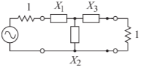
Figure \(\PageIndex{1}\)

1. Design an LPF with \(\omega_{c} = 1\text{ rad/s}\), \(Z_{0} =1\:\Omega\).
2. Design a HPF with \(\omega_{c} = 1\text{ rad/s}\), \(Z_{0} =1\:\Omega\).
3. Design a HPF with \(f_{c} = 1\text{ GHz}\), \(Z_{0} =1\:\Omega\).
4. Design a HPF with \(f_{c} = 1\text{ GHz}\), \(Z_{0} = 50\:\Omega\).

21. This problem considers the design of a Butterworth bandpass filter at \(900\text{ MHz}\).
    1. Design an \(LC\) second-order Butterworth lowpass filter with a corner frequency of \(1\text{ rad/s}\) in a \(1\:\Omega\) system.
    2. Using the above filter prototype, design a lowpass filter with a corner frequency of \(900\text{ MHz}\).
    3. Design a second-order Butterworth bandpass filter at \(900\text{ MHz}\) using the lowpass filter prototype in (a). Use a fractional bandwidth of \(0.1\) and a system impedance of \(50\:\Omega\).
    4. What is the \(3\text{ dB}\) bandwidth of the filter in (c)?
22. Design a third-order maximally flat bandpass filter prototype in a \(50\:\Omega\) system centered at \(1\text{ GHz}\) with a \(10\%\) bandwidth. The lowpass prototype of a third-order maximally flat filter is shown in Figure 2.6.3.
    1. Convert the prototype lowpass filter to a lowpass filter with inverters and capacitors only; that is, remove the series inductors.
    2. Scale the filter to take the corner frequency from \(1\text{ rad/s}\) to \(1\text{ GHz}\).
    3. Transform the lowpass filter into a bandpass filter. That is, replace each shunt capacitor by a parallel \(LC\) network. This step will establish the bandwidth of the filter.
    4. Transform the system impedance of the filter from \(1\) to \(50\:\Omega\).
23. The lowpass prototype of a fourth-order lowpass Butterworth filter is shown below. The corner frequency is \(1\text{ rad/s}\).

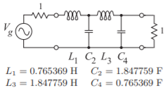
Figure \(\PageIndex{2}\)

Based on this, develop a fourth-order Butterworth bandpass filter prototype centered at \(10^{9}\text{ rad/s}\) with a fractional bandwidth of \(5\%\).

1. Scale the lowpass prototype to have a corner frequency of \(10^{9}\text{ rad/s}\). Draw the prototype with element values.
2. Draw the schematic of the lumped-element fourth-order Butterworth bandpass prototype based on the original lowpass filter prototype.
3. Derive the element values of the lumped-element bandpass filter prototype in a \(75\:\Omega\) system.

24. Design a third-order Type \(2\) Chebyshev highpass filter with a corner frequency of \(1\text{ GHz}\), a system impedance of \(50\:\Omega\), and \(0.2\text{ dB}\) ripple. There are a number of steps in the design, and to demonstrate that you understand them you are asked to complete the table below. For each stage of the filter synthesis you must indicate whether the element is an inductance or a capacitance by writing \(L\) or \(C\) in the appropriate cell. Other cells require a numeric value and you must include units. The \(X\) element is identified in the prototype below. A Cauer \(2\) lowpass filter prototype is shown with ωc being the corner radian frequency, \(f_{c} = \omega_{c}/(2\pi )\) being the corner frequency, and \(Z_{0}\) being the system impedance.

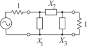
Figure \(\PageIndex{3}\)

1. Complete the LPF (lowpass filter) column of the table with \(\omega_{c} = 1\text{ rad/s}\), \(Z_{0} =1\:\Omega\).
2. Complete the HPF (highpass filter) column of the table with \(\omega_{c} = 1\text{ rad/s}\), \(Z_{0} =1\:\Omega\).
3. Complete the second HPF column of the table with \(f_{c} = 1\text{ GHz}\), \(Z_{0} =1\:\Omega\).
4. Complete the third HPF column of the table with \(f_{c} = 1\text{ GHz}\), \(Z_{0} = 50\:\Omega\).

ELEMENT	LPF
	\(\omega_{c}=1\text{ rad/s}\), \(Z_{0}=1\:\Omega\)
	\(L\) or \(C\)	Value (units)
\(X_{1}\)
\(X_{2}\)
\(X_{3}\)

Table \(\PageIndex{1}\)

ELEMENT	HPF
	\(\omega_{c}=1\text{ rad/s}\), \(Z_{0}=1\:\Omega\)
	\(L\) or \(C\)	Value (units)
\(X_{1}\)
\(X_{2}\)
\(X_{3}\)

Table \(\PageIndex{2}\)

ELEMENT	HPF
	\(f_{c}=1\text{ GHz}\), \(Z_{0}=1\:\Omega\)
	\(L\) or \(C\)	Value (units)
\(X_{1}\)
\(X_{2}\)
\(X_{3}\)

Table \(\PageIndex{3}\)

ELEMENT	HPF
	\(f_{c}=1\text{ GHz}\), \(Z_{0}=50\:\Omega\)
	\(L\) or \(C\)	Value (units)
\(X_{1}\)
\(X_{2}\)
\(X_{3}\)

Table \(\PageIndex{4}\)

25. What is the input impedance of a shorted \(\lambda /8\) long transmission line with a characteristic impedance of \(Z_{0}\)?
26. What is the input impedance of an open-circuited \(\lambda /8\) long transmission line with a characteristic impedance of \(Z_{0}\)?
27. Apply Richards’s transformation to a shunt inductor with a reactance of \(50\:\Omega\). What is the electrical length of the shorted stub if the stub has a characteristic impedance of \(50\:\Omega\)?
28. Apply Richards’s transformation to a shunt capacitor with a reactance of \(−50\:\Omega\). What is the characteristic impedance of the open-circuited stub if the electrical length of the stub is one-quarter wavelength long?

2.12.1 Exercises by Section

\(†\)challenging, \(‡\)very challenging

\(§2.2\: 1†, 2\)

\(§2.4\: 3†, 4†\)

\(§2.5\: 5†\)

\(§2.6\: 6†, 7†, 8†, 9†\)

\(§2.7\: 10, 11†, 12†\)

\(§2.8\: 13, 14†, 15†, 16†, 17†, 18†, 19†\)

\(§2.9\: 20†, 21†, 2†2, 23†, 24†\)

\(§2.12\: 25, 26, 27†, 28†\)

2.12.2 Answers to Selected Exercises

1. (c) \(\Gamma(s)=\frac{s^{2}}{s^{2}+\sqrt{2}s+1}\)
2. \(|T(w)|^{2}=1/(1+\omega^{8})\)
3. (f) \(\begin{array}{l}{−0.38 + \jmath 0.92} \\ {−0.38 -\jmath 0.92} \\ {−0.92 + \jmath 0.38} \\ {-0.38-\jmath 0.92}\end{array}\)

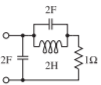
Figure \(\PageIndex{4}\)

13. (c) \(9\)
14. (a) \(\left[\begin{array}{cc}{1}&{sC(50)^{2}}\\{0}&{1}\end{array}\right]\)

17. \(889\text{ fF}\)
18. \(10\text{ nH}\)
19. (c) \(-Z_{2}=-\jmath 50\:\Omega\)

24. \(1\text{ GHz},\: 50\:\Omega,\: \text{HPF}: X_{3}=6.5\text{ nH}\)