
6.9: Phase Locked Loop (PLL)
- Page ID
- 46147
\( \newcommand{\vecs}[1]{\overset { \scriptstyle \rightharpoonup} {\mathbf{#1}} } \)
\( \newcommand{\vecd}[1]{\overset{-\!-\!\rightharpoonup}{\vphantom{a}\smash {#1}}} \)
\( \newcommand{\id}{\mathrm{id}}\) \( \newcommand{\Span}{\mathrm{span}}\)
( \newcommand{\kernel}{\mathrm{null}\,}\) \( \newcommand{\range}{\mathrm{range}\,}\)
\( \newcommand{\RealPart}{\mathrm{Re}}\) \( \newcommand{\ImaginaryPart}{\mathrm{Im}}\)
\( \newcommand{\Argument}{\mathrm{Arg}}\) \( \newcommand{\norm}[1]{\| #1 \|}\)
\( \newcommand{\inner}[2]{\langle #1, #2 \rangle}\)
\( \newcommand{\Span}{\mathrm{span}}\)
\( \newcommand{\id}{\mathrm{id}}\)
\( \newcommand{\Span}{\mathrm{span}}\)
\( \newcommand{\kernel}{\mathrm{null}\,}\)
\( \newcommand{\range}{\mathrm{range}\,}\)
\( \newcommand{\RealPart}{\mathrm{Re}}\)
\( \newcommand{\ImaginaryPart}{\mathrm{Im}}\)
\( \newcommand{\Argument}{\mathrm{Arg}}\)
\( \newcommand{\norm}[1]{\| #1 \|}\)
\( \newcommand{\inner}[2]{\langle #1, #2 \rangle}\)
\( \newcommand{\Span}{\mathrm{span}}\) \( \newcommand{\AA}{\unicode[.8,0]{x212B}}\)
\( \newcommand{\vectorA}[1]{\vec{#1}} % arrow\)
\( \newcommand{\vectorAt}[1]{\vec{\text{#1}}} % arrow\)
\( \newcommand{\vectorB}[1]{\overset { \scriptstyle \rightharpoonup} {\mathbf{#1}} } \)
\( \newcommand{\vectorC}[1]{\textbf{#1}} \)
\( \newcommand{\vectorD}[1]{\overrightarrow{#1}} \)
\( \newcommand{\vectorDt}[1]{\overrightarrow{\text{#1}}} \)
\( \newcommand{\vectE}[1]{\overset{-\!-\!\rightharpoonup}{\vphantom{a}\smash{\mathbf {#1}}}} \)
\( \newcommand{\vecs}[1]{\overset { \scriptstyle \rightharpoonup} {\mathbf{#1}} } \)
\( \newcommand{\vecd}[1]{\overset{-\!-\!\rightharpoonup}{\vphantom{a}\smash {#1}}} \)
\(\newcommand{\avec}{\mathbf a}\) \(\newcommand{\bvec}{\mathbf b}\) \(\newcommand{\cvec}{\mathbf c}\) \(\newcommand{\dvec}{\mathbf d}\) \(\newcommand{\dtil}{\widetilde{\mathbf d}}\) \(\newcommand{\evec}{\mathbf e}\) \(\newcommand{\fvec}{\mathbf f}\) \(\newcommand{\nvec}{\mathbf n}\) \(\newcommand{\pvec}{\mathbf p}\) \(\newcommand{\qvec}{\mathbf q}\) \(\newcommand{\svec}{\mathbf s}\) \(\newcommand{\tvec}{\mathbf t}\) \(\newcommand{\uvec}{\mathbf u}\) \(\newcommand{\vvec}{\mathbf v}\) \(\newcommand{\wvec}{\mathbf w}\) \(\newcommand{\xvec}{\mathbf x}\) \(\newcommand{\yvec}{\mathbf y}\) \(\newcommand{\zvec}{\mathbf z}\) \(\newcommand{\rvec}{\mathbf r}\) \(\newcommand{\mvec}{\mathbf m}\) \(\newcommand{\zerovec}{\mathbf 0}\) \(\newcommand{\onevec}{\mathbf 1}\) \(\newcommand{\real}{\mathbb R}\) \(\newcommand{\twovec}[2]{\left[\begin{array}{r}#1 \\ #2 \end{array}\right]}\) \(\newcommand{\ctwovec}[2]{\left[\begin{array}{c}#1 \\ #2 \end{array}\right]}\) \(\newcommand{\threevec}[3]{\left[\begin{array}{r}#1 \\ #2 \\ #3 \end{array}\right]}\) \(\newcommand{\cthreevec}[3]{\left[\begin{array}{c}#1 \\ #2 \\ #3 \end{array}\right]}\) \(\newcommand{\fourvec}[4]{\left[\begin{array}{r}#1 \\ #2 \\ #3 \\ #4 \end{array}\right]}\) \(\newcommand{\cfourvec}[4]{\left[\begin{array}{c}#1 \\ #2 \\ #3 \\ #4 \end{array}\right]}\) \(\newcommand{\fivevec}[5]{\left[\begin{array}{r}#1 \\ #2 \\ #3 \\ #4 \\ #5 \\ \end{array}\right]}\) \(\newcommand{\cfivevec}[5]{\left[\begin{array}{c}#1 \\ #2 \\ #3 \\ #4 \\ #5 \\ \end{array}\right]}\) \(\newcommand{\mattwo}[4]{\left[\begin{array}{rr}#1 \amp #2 \\ #3 \amp #4 \\ \end{array}\right]}\) \(\newcommand{\laspan}[1]{\text{Span}\{#1\}}\) \(\newcommand{\bcal}{\cal B}\) \(\newcommand{\ccal}{\cal C}\) \(\newcommand{\scal}{\cal S}\) \(\newcommand{\wcal}{\cal W}\) \(\newcommand{\ecal}{\cal E}\) \(\newcommand{\coords}[2]{\left\{#1\right\}_{#2}}\) \(\newcommand{\gray}[1]{\color{gray}{#1}}\) \(\newcommand{\lgray}[1]{\color{lightgray}{#1}}\) \(\newcommand{\rank}{\operatorname{rank}}\) \(\newcommand{\row}{\text{Row}}\) \(\newcommand{\col}{\text{Col}}\) \(\renewcommand{\row}{\text{Row}}\) \(\newcommand{\nul}{\text{Nul}}\) \(\newcommand{\var}{\text{Var}}\) \(\newcommand{\corr}{\text{corr}}\) \(\newcommand{\len}[1]{\left|#1\right|}\) \(\newcommand{\bbar}{\overline{\bvec}}\) \(\newcommand{\bhat}{\widehat{\bvec}}\) \(\newcommand{\bperp}{\bvec^\perp}\) \(\newcommand{\xhat}{\widehat{\xvec}}\) \(\newcommand{\vhat}{\widehat{\vvec}}\) \(\newcommand{\uhat}{\widehat{\uvec}}\) \(\newcommand{\what}{\widehat{\wvec}}\) \(\newcommand{\Sighat}{\widehat{\Sigma}}\) \(\newcommand{\lt}{<}\) \(\newcommand{\gt}{>}\) \(\newcommand{\amp}{&}\) \(\definecolor{fillinmathshade}{gray}{0.9}\)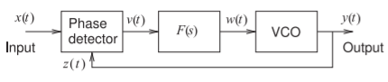
Figure \(\PageIndex{1}\): A phase-locked loop with a phase-detector and a frequency divider indicated by \((1/N)\).
A phase-locked loop (PLL) is a feedback system in which the frequency and phase of an output signal is related to the frequency and phase of an input signal. The block diagram of a PLL is shown in Figure \(\PageIndex{1}\). An input signal \(x(t)\) is compared to a feedback signal \(z(t)\). The frequency of \(y(t)\) will be the average frequency of \(x(t)\). The way the loop achieves this is that the output of the phase detector is proportional to the phase difference of \(x(t)\) and \(z(t)\). This is then filtered by the block \(F(s)\) (generally a lowpass filter) to produce a DC-like signal that drives a VCO. The filtering block, \(F(s)\), removes undesired components from the phase detector and also sets the dynamic response of the PLL.
6.9.1 Operation
The operation of the PLL in Figure \(\PageIndex{1}\) can be modeled as a linear system with the assumption that \(x(t)\) and \(z(t) (= y(t)\) here) are nearly periodic signals. Thus, approximately
\[\label{eq:1}x(t)=A_{x}\cos(\omega_{x}t+\phi_{x})\quad\text{and}\quad z(t)=A_{w}\cos(\omega_{z}t+\phi_{z}) \]
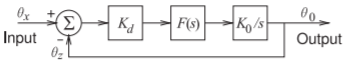
Figure \(\PageIndex{2}\): Linearized model of an analog phase-locked loop.
PLLs require that the radian frequency \(\omega_{x}\) be close to \(\omega_{z}\), which is near the free-running frequency of the VCO. (In practice, \(\omega_{x}\) is usually much less than \(\omega_{z}\) and a frequency divider is used to divide the signal at \(\omega_{z}\) to obtain a signal with a frequency close to \(\omega_{x}\). The analysis is similar to that presented here.) This defines the capture range of the PLL. Therefore Equation \(\eqref{eq:1}\) can be written
\[\label{eq:2}x(t)=A_{x}\cos(\Theta_{x}(t))\quad\text{and}\quad z(t)=A_{w}\cos(\Theta_{0}(t)) \]
The phases \(\Theta_{x}\) and \(\Theta_{0}\) incorporate the original phases \(\phi_{x}\) and \(\phi_{w}\), respectively, and the effective time-dependent phase difference due to the small time-dependent difference of the frequencies of \(x(t)\) and \(z(t)\). Analysis of the PLL in Figure \(\PageIndex{1}\) begins with the voltage at the output of the phase detector, \(v(t)\), which is proportional to the phase difference of the two input signals and independent of their amplitude:
\[\label{eq:3}v(t)=K_{d}(\Theta_{x}-\Theta_{0}) \]
where \(K_{d}\) is the phase detector gain factor. The output of the phase detector is filtered by the block with transfer function \(F(s)\). Usually this block is a lowpass filter, but there are applications where it could be a bandpass filter or have some other characteristic.
The output of the VCO is controlled by the voltage \(w(t)\) producing a signal with frequency
\[\label{eq:4}f_{0}=f_{c}+\Delta f = f_{c}+K_{0}v(t) \]
where \(f_{c}\) is the frequency of oscillation when the control voltage is zero and \(K_{0}\) is the VCO gain factor.
Equations \(\eqref{eq:3}\) and \(\eqref{eq:4}\) describe the linear system shown in Figure \(\PageIndex{2}\). The transfer function of this system is
\[\label{eq:5}\frac{\theta_{0}}{\theta_{x}}=\frac{K_{d}K_{0}F(s)/s}{1+K_{d}K_{0}F(s)/s}=\frac{G(s)}{1+G(s)} \]
where \(G(s) = K_{d}K_{0}F(s)\). The phase error function is
\[\label{eq:6}\epsilon(s)=\theta_{x}(s)-\theta_{0}=\theta_{x}\left[1-\frac{K_{d}K_{0}F(s)}{s+K_{d}K_{0}F(s)}\right]=\frac{s\theta_{x}(s)}{s+K_{d}K_{0}F(s)} \]
So the phase error function is directly related to the phase of the input signal \(x(t)\). In the next section a particular choice of the transfer function \(F(s)\) is used, leading to the identification of a particular PLL application.
6.9.2 First-Order PLL
Without a filter (i.e., \(F(s) = 1\)) the PLL is referred to as a first-order PLL or first-order loop and its transfer function is
\[\label{eq:7}\frac{\theta_{0}(s)}{\theta_{x}(0)}=\frac{K_{d}K_{0}/s}{1+K_{d}K_{0}/s}=\frac{K_{d}K_{0}}{s+K_{d}K_{0}} \]
This seems to be the transfer function of a lowpass filter, but the input to the system is phase and the output is the phase deviation from the free-running frequency of the VCO. The phase error function of the first-order PLL is
\[\label{eq:8}\epsilon (s)=\theta_{x}(s)-\theta_{0}=\theta_{x}(s)\left(1-\frac{K_{d}K_{0}}{s+K_{d}K_{0}}\right)=\frac{s\theta_{x}(s)}{s+K_{d}K_{0}} \]
The steady-state response of the first-order PLL to specific input signals will now be derived. The long-term (steady-state) behavior is developed using the final-value theorem. A function \(H(s)\) with all poles in the left-half plane has a time-domain response \(h(t)\) with long-term behavior given by
\[\label{eq:9}\lim_{t\to\infty}h(t)=\lim_{s\to 0}sH(s) \]
Consider now the response to a step change, \(\Delta\theta_{x}\), of the phase of the input signal. The Laplace transform of a step function of magnitude \(\Delta\theta_{x}\) is \(\Delta\theta_{x}/s\) and this is what is used in Equation \(\eqref{eq:8}\). Thus the steady-state error function, \(\epsilon_{ss} = \epsilon (t)\) as \(t\to\infty\), is
\[\begin{align}\epsilon_{ss}&=\lim_{s\to 0}\left[\frac{s^{2}\theta_{x}(s)}{s+K_{d}K_{0}}\right]=\lim_{s\to 0}\left[\frac{s^{2}\Delta\theta_{x}/s}{s+K_{d}K_{0}}\right]=\lim_{s\to 0}\left[\frac{s\Delta\theta_{x}}{s+K_{d}K_{0}}\right]\nonumber \\ \label{eq:10}&=0\end{align} \]
Equation \(\eqref{eq:10}\) indicates that a first-order PLL will eventually track a phase change of the input signal. However, it will not respond immediately as the loop has a lowpass characteristic. In effect the PLL is acting as a high-\(Q\) bandpass filter.
Now consider a step change in the frequency of the input signal. If the step change in the radian frequency of \(x(t)\) is \(\Delta\omega_{x}\), then the resulting phase change will be a ramp so that, in the Laplace domain, \(\theta (s)=\Delta\omega_{x}/s^{2}\). Then the steady-state error is
\[\begin{align}\epsilon_{ss}&=\lim_{s\to 0}\left[\frac{s^{2}\Delta\omega_{x}/s^{2}}{s+K_{d}K_{0}}\right] = \lim_{s\to 0}\left[\frac{\Delta\omega_{x}}{s+K_{d}K_{0}}\right]\nonumber \\ \label{eq:11}&=\Delta\omega_{x}/(K_{d}K_{0})\end{align} \]
Equation \(\eqref{eq:11}\) indicates that a first-order PLL will follow a change in frequency with a phase error that is proportional to the magnitude of the frequency change. So if the input signal \(x(t)\) is a frequency modulated signal, the first-order PLL will demodulate the signal and recover the original modulation as the error signal. Thus a first-order PLL demodulates an FM signal, that is, it is a frequency demodulator.
6.9.3 Applications
Three applications of the PLL are shown in Figure \(\PageIndex{3}\). A frequency synthesizer is used to create a signal locked to a fixed-frequency and very accurate reference oscillator but at another frequency (see Figure \(\PageIndex{3}\)(a)). Typically the reference is a precision low-frequency reference oscillator, such as a quartz crystal oscillator [36]. The output frequency is not at the same frequency as the reference oscillator. This is accomplished by including a frequency divider in the PLL. Normally the division factor, \(N\), is an integer
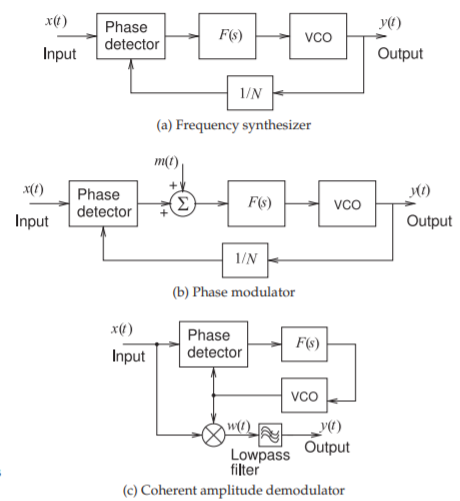
Figure \(\PageIndex{3}\): Applications using phase-locked loops.
so that the output signal’s frequency will be an integer multiple of the input frequency. A fractional-\(N\) frequency synthesizer is achieved using two integer dividers with division factors \(N\) and \(M\). A controller alternates between the two division factors so that the VCO tends to output first one frequency and then the next. The VCO stabilizes at a frequency that is the weighted average of the two division factors. If the frequency is divided by \(M\) for a time \(\tau_{M}\), then by \(N\) for time \(\tau_{N}\), and repeated, then the effective division factor is \((\tau_{M}M + \tau_{N}N)/(\tau_{M} +\tau_{N})\). The loop dynamics (determined by the filter \(F(s)\)) is chosen so that the VCO can only change more slowly than the toggling of the division factors. The division factors, and the toggling between its two values, are chosen to synthesize an output signal with the desired frequency.
The second application of the PLL is a phase modulator, see Figure \(\PageIndex{3}\)(b). The phase modulating signal \(m(t)\) effectively is adding to the phase error generated by the phase detector. This results in a change in the phase of the VCO output compensating for the inserted phase change.
The third application of the PLL is the coherent amplitude demodulator shown in Figure \(\PageIndex{3}\)(c). The input is an amplitude modulated signal
\[\label{eq:12}x(t)=A[1+m(t)]\sin(\omega_{0}t) \]
which is demodulated to recover \(m(t)\) by multiplying \(x(t)\) by an LO signal with the same carrier frequency. The characteristic of \(F(s)\) is chosen so that the PLL generates the LO signal as the loop establishes the oscillation
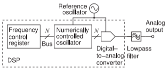
Figure \(\PageIndex{4}\): Direct digital synthesis (DDS) module.
frequency as the central frequency of the modulated input. The loop filter \(F(s)\) ensures that the VCO frequency cannot change too quickly and the output frequency of the VCO approximates a sinusoidal signal having a radian frequency \(\omega_{0}\) with a phase offset. Thus
\[\label{eq:13} w(t)=x(t)\sin(\omega_{0}t+\theta)=A[1+m(t)]\frac{1}{2}[\cos\theta -\cos(2\omega_{0}t_{\theta})] \]
Following lowpass filtering the output is
\[\label{eq:14}y(t)=A[1+m(t)]\cos\theta \]
With loop dynamics chosen so that \(\theta\) is small, the original modulation, \(m(t)\), is recovered. This AM demodulator performs well when the input SNR is low as demodulation is coherent.