11.2: Filter Types

No matter how a filter is realized, it will usually conform to one of four basic response types. These types are: high-pass, low-pass, band-pass, and band-reject (also known as a notch type). A high-pass filter allows only frequencies above a certain break point to pass through. In other words, it attenuates low frequency components. Its general amplitude frequency response is shown in Figure \(\PageIndex{1}\). A low-pass filter is the logical mirror of the high-pass, that is, it allows only low frequency signals to pass through, while suppressing high-frequency components. Its response is shown in Figure \(\PageIndex{2}\). The band-pass filter can be thought of as a combination of high- and low-pass filters. It only allows frequencies within a specified range to pass through. Its logical inverse is the band-reject filter that allows everything to pass through, with the exception of a specific range of frequencies. The amplitude frequency response plots for these last two types are shown in Figures \(\PageIndex{3}\) and \(\PageIndex{4}\), respectively. In complex systems, it is possible to combine several different types together in order to achieve a desired overall response characteristic.

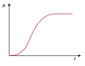
Figure \(\PageIndex{1}\): High-pass response.

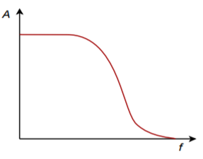
Figure \(\PageIndex{2}\): Low-pass response.

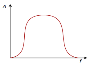
Figure \(\PageIndex{3}\): Band-pass response.

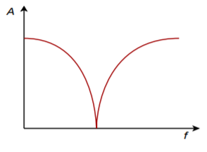
Figure \(\PageIndex{4}\): Notch response.

In each plot, there are three basic regions. The flat area where the input signal is allowed to pass through is known as the pass band. The edge of the pass band is denoted by the break frequency. The break frequency is usually defined as the point at which the response has fallen 3 dB from its pass-band value. Consequently, it is also referred to as the dB down frequency. It is important to note that the break frequency is not} always equal to the natural critical frequency, \(f_c\). The area where the input signal is fully suppressed is called the stop band. The section between the pass band and the stop band is referred to as the transition band. This is shown for the low-pass filter in Figure \(\PageIndex{5}\). Note that plots \(\PageIndex{1}\) through \(\PageIndex{4}\) only define the general response of the filters. The actual shape of the transition band for a given design will be refined in following sections.

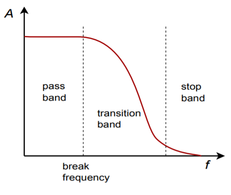
Figure \(\PageIndex{5}\): Filter regions.

These response plots may be achieved through the use of simple RLC circuits. For example, the simple lag network shown in Figure \(\PageIndex{6}\) may be classified as a low-pass filter. You know from earlier work that lag networks attenuate high frequencies. In a similar vein, a band-pass filter may be constructed as shown in Figure \(\PageIndex{7}\). Note that at resonance, the tank circuit exhibits an impedance peak, whereas the series combination exhibits its minimum impedance. Therefore, a large portion of \(V_{in}\) will appear at \(V_{out}\). At very high or low frequencies the situation is reversed (the parallel combination shows a low impedance, and the series combination shows a high impedance), and very little of \(V_{in}\) appears at the output. Note that no active components are used in this circuit. This is a passive filter.

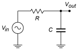
Figure \(\PageIndex{6}\): Passive low-pass filter.

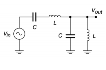
Figure \(\PageIndex{7}\): Passive band-pass filter.