11.8: Notch Filter (Band-Reject) Realizations

Last updated
Save as PDF

Page ID: 26749

\( \newcommand{\vecs}[1]{\overset { \scriptstyle \rightharpoonup} {\mathbf{#1}} } \) \( \newcommand{\vecd}[1]{\overset{-\!-\!\rightharpoonup}{\vphantom{a}\smash {#1}}} \)\(\newcommand{\id}{\mathrm{id}}\) \( \newcommand{\Span}{\mathrm{span}}\) \( \newcommand{\kernel}{\mathrm{null}\,}\) \( \newcommand{\range}{\mathrm{range}\,}\) \( \newcommand{\RealPart}{\mathrm{Re}}\) \( \newcommand{\ImaginaryPart}{\mathrm{Im}}\) \( \newcommand{\Argument}{\mathrm{Arg}}\) \( \newcommand{\norm}[1]{\| #1 \|}\) \( \newcommand{\inner}[2]{\langle #1, #2 \rangle}\) \( \newcommand{\Span}{\mathrm{span}}\) \(\newcommand{\id}{\mathrm{id}}\) \( \newcommand{\Span}{\mathrm{span}}\) \( \newcommand{\kernel}{\mathrm{null}\,}\) \( \newcommand{\range}{\mathrm{range}\,}\) \( \newcommand{\RealPart}{\mathrm{Re}}\) \( \newcommand{\ImaginaryPart}{\mathrm{Im}}\) \( \newcommand{\Argument}{\mathrm{Arg}}\) \( \newcommand{\norm}[1]{\| #1 \|}\) \( \newcommand{\inner}[2]{\langle #1, #2 \rangle}\) \( \newcommand{\Span}{\mathrm{span}}\)\(\newcommand{\AA}{\unicode[.8,0]{x212B}}\)

By summing the high-pass and low-pass outputs of the state-variable filter, a notch, or band-reject, filter may be formed. Filters of this type are commonly used to remove interference signals. The summation is easily performed with a simple parallel-parallel summing amplifier, as shown in Figure \(\PageIndex{1}\).

11.8.1.png

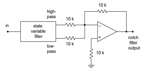
Figure \(\PageIndex{1}\): Notch filter.

For reasonable \(Q\) values, there will be tight correlation between the calculated band-pass center and −3 dB frequencies, and the notch center and −3 dB frequencies. The component calculations proceed as in the band-pass filter.

Example \(\PageIndex{1}\)

A filter is needed to remove induced 60 Hz hum from a transducer's signal. The rejection bandwidth of the filter should be no more than 2 Hz. From the specifications we know that the center frequency is 60 Hz and the \(Q\) is 60/2, or 30. For simplicity, we will use the fixed-gain form. (Note that the gain of the filter on either side of the notch will be unity.)

\[R_{damping} = 3Q−1 \\ R_{damping} = 3\times 30−1 \\ R_{damping} = 89\Omega \nonumber \]

\[\omega_o = 2 \pi 60 \\ \omega_o = 377 rad/s \nonumber \]

Scaling \(C\) produces

\[C = \frac{1}{377} \\ C = 2.65 \text{ milliFarads} \nonumber \]

A practical value scaling of \(10^4\) produces the circuit of Figure \(\PageIndex{2}\). Note that the damping resistors have only been scaled by \(10^3\), as an \(R_{damping}\) value of \(890 k\Omega\) might be excessive. Remember, it is the ratio of these two resistors that is important, not their absolute values.

11.8.2.png

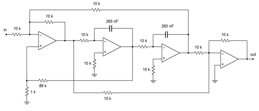
Figure \(\PageIndex{2}\): Completed notch filter for Example \(\PageIndex{1}\).

Computer Simulation

Figure \(\PageIndex{3}\) shows a simulation of the circuit of Example \(\PageIndex{1}\) using Multisim. To keep the layout simple, an ideal op amp model was chosen. The AC analysis shows the very sharp notch centered at 60 Hz as expected. As filters of this type are designed to remove a single frequency without affecting surrounding material, high precision tuning components are required. To see the effects of even modest component deviations in a production run, a Monte Carlo analysis proves invaluable. In Figure \(\PageIndex{3c}\) a series of 10 runs is shown. Each resistor and capacitor in the filter has been given a 1 percent nominal tolerance. Further, the frequency plot range has been narrowed down to just 10 hertz on either side of the target frequency. Even with these relatively tight tolerances, tuning deviations of more than 1 hertz can be seen. Also, the response shape is not perfectly symmetrical in all cases.

11.8.3.png

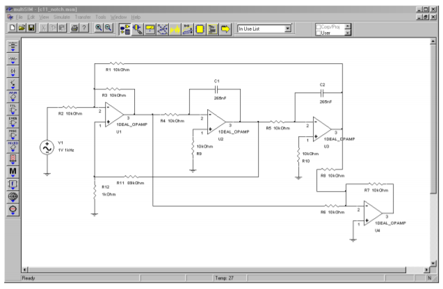
Figure \(\PageIndex{3a}\): State-variable notch filter in Multisim.

11.8.4.png

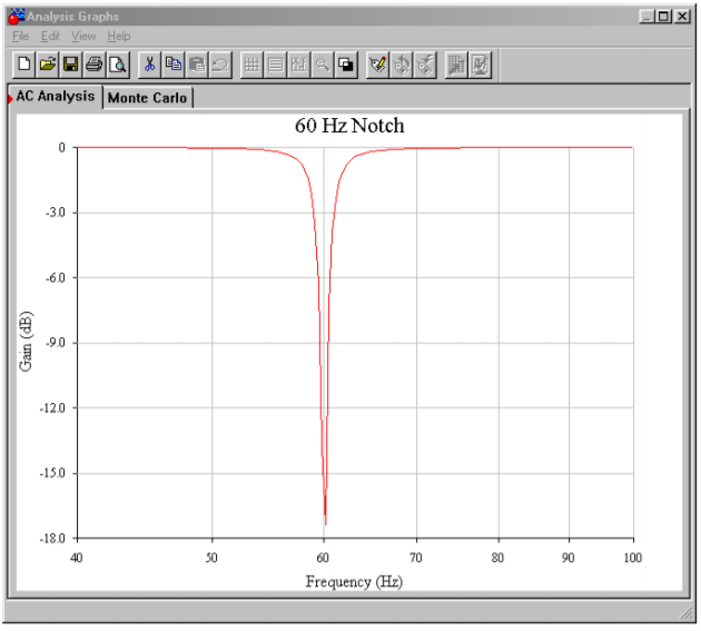
Figure \(\PageIndex{3b}\): Ideal notch response.

11.8.5.png

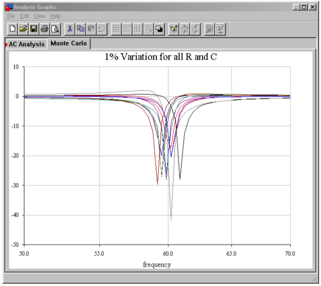
Figure \(\PageIndex{3c}\): Typical response with 1% component variations.

A Note on Component Selection

Ideally, the circuit of Example \(\PageIndex{1}\) will produce −3 dB points at approximately 59 Hz and 61 Hz and will infinitely attenuate 60 Hz tones. In reality, component tolerances may alter the response and, therefore, high-quality parts are required for accurate, high- \(Q\) circuits such as this. Even simpler, less-demanding circuits such as a second-order Sallen and Key filter may not perform as expected if lower quality parts are used. As a general rule, component accuracy and stability becomes more important as filter \(Q\) and order increase. One percent tolerance metal film resistors are commonly used, with 5 percent carbon film types being satisfactory for the simpler circuits. For capacitors, film types such as polyethylene (mylar) are common for general-purpose work, with polycarbonate, polystyrene, polypropylene, and teflon being used for the more stringent requirements. For small capacitance values (<100 pF), NPO ceramics may be used. Generally, large ceramic disc and aluminum electrolytic capacitors are avoided due to their wide tolerance and instability with temperature, applied voltage, and other factors.

11.8.1: Filter Design Tools

In order to further speed the process of active filter design, some manufacturers offer free filter design software. Examples include FilterCAD from Linear Technology and FilterPro from Burr-Brown. Some programs are rather generic and help you design Sallen and Key, multiple-feedback, and state-variable filters. Others are written expressly to support the manufacturer's specialized filter ICs. Typically, the programs will print out component values given desired filter types and break frequencies. Bode plots and pulse waveform simulations may also be available. Such programs can certainly reduce design tedium.