
5.7: Exercises
- Page ID
- 34245

Unless otherwise specified, use \(\beta\) = 100.
5.7.1: Analysis Problems
1. Plot the load line for the circuit of Figure \(\PageIndex{1}\). \(V_{CC}\) = 20 V, \(V_{EE}\) = −8 V, \(R_B\) = 7.5 k\(\Omega\), \(R_E\) = 10 k\(\Omega\), \(R_C\) = 12 k\(\Omega\).
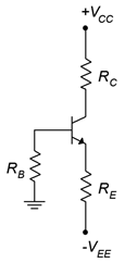
Figure \(\PageIndex{1}\)
2. Determine the new Q point for Problem 1 if \(\beta\) = 250.
3. Plot the load line for the circuit of Figure \(\PageIndex{2}\). \(V_{EE}\) = 5 V, \(V_{CC}\) = −18 V, \(R_B\) = 22 k\(\Omega\), \(R_E\) = 1.2 k\(\Omega\), \(R_C\) = 1.5 k\(\Omega\).
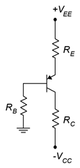
Figure \(\PageIndex{2}\)
4. Determine the new Q point for Problem 3 if \(\beta\) = 50.
5. Plot the load line for the circuit of Figure \(\PageIndex{3}\). \(V_{CC}\) = 20 V, \(R_1\) = 15 k\(\Omega\), \(R_2\) = 5 k\(\Omega\), \(R_E\) = 4.3 k\(\Omega\), \(R_C\) = 9.1 k\(\Omega\).
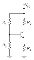
Figure \(\PageIndex{3}\)
6. Determine the new Q point for Problem 5 if \(\beta\) = 150.
7. Plot the load line for the circuit of Figure \(\PageIndex{4}\). \(V_{EE}\) = 16 V, \(R_1\) = 12 k\(\Omega\), \(R_2\) = 4.7 k\(\Omega\), \(R_E\) = 6.2 k\(\Omega\), \(R_C\) = 10 k\(\Omega\).
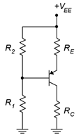
Figure \(\PageIndex{4}\)
8. Determine the new Q point for Problem 7 if \(\beta\) = 200.
9. Plot the load line for the circuit of Figure \(\PageIndex{5}\). \(V_{CC}\) = 12 V, \(R_B\) = 560 k\(\Omega\), \(R_C\) = 3.3 k\(\Omega\).
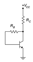
Figure \(\PageIndex{5}\)
10. Determine the new Q point for Problem 9 if \(\beta\) = 75.
11. Plot the load line for the circuit of Figure \(\PageIndex{6}\).
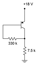
Figure \(\PageIndex{6}\)
12. Determine the new Q point for Problem 11 if \(\beta\) = 200.
13. Plot the load line for the circuit of Figure \(\PageIndex{7}\). \(V_{CC}\) = 15 V, \(R_B\) = 470 k\(\Omega\), \(R_E\) = 560 \(\Omega\), \(R_C\) = 3.3 k\(\Omega\).
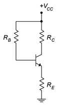
Figure \(\PageIndex{7}\)
14. Determine the new Q point for Problem 13 if \(\beta\) = 170.
15. Plot the load line for the circuit of Figure \(\PageIndex{8}\).
16. Determine the new Q point for Problem 15 if \(\beta\) = 75.
17. Plot the load line for the circuit of Figure \(\PageIndex{9}\). \(V_{EE}\) = 18 V, \(R_B\) = 680 k\(\Omega\), \(R_E\) = 270 \(\Omega\), \(R_C\) = 3.9 k\(\Omega\).
18. Determine the new Q point for Problem 17 if \(\beta\) = 200.
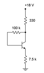
Figure \(\PageIndex{8}\)
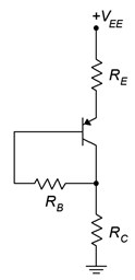
Figure \(\PageIndex{9}\)
5.7.2: Design Problems
19. Determine a value for \(R_E\) in the circuit of Figure \(\PageIndex{1}\) to set \(I_C\) = 2 mA. Use \(V_{CC}\) = 20 V, \(V_{EE}\) = −8 V, \(R_B\) = 10 k\(\Omega\), \(R_C\) = 5.6 k\(\Omega\).
20. Determine a value for \(R_C\) in the circuit of Figure \(\PageIndex{2}\) to set \(V_{CE}\) = 10 V. Use \(V_{CC}\) = −25 V, \(V_{EE}\) = 6 V, \(R_B\) = 15 k\(\Omega\), \(R_E\) = 6.8 k\(\Omega\).
21. Determine a value for \(R_C\) in the circuit of Figure \(\PageIndex{3}\) to set \(V_{CE}\) = 8 V. Use \(V_{CC}\) = 24 V, \(R_1\) = 22 k\(\Omega\), \(R_2\) = 10 k\(\Omega\), \(R_E\) = 5.6 k\(\Omega\).
22. Determine new values for \(R_1\) and \(R_2\) in the circuit of Figure \(\PageIndex{4}\) in order to set \(I_C\) = 500 \(\mu\)A. \(V_{EE}\) = 22 V, \(R_E\) = 15 k\(\Omega\), \(R_C\) = 6.8 k\(\Omega\).
5.7.3: Challenge Problems
23. Determine the maximum and minimum values for \(I_C\) in Problem 1 if every resistor has a 10% tolerance.
24. Determine the maximum and minimum values for \(V_{CE}\) in Problem 3 if every resistor has a 5% tolerance.
25. Determine a value for \(R_E\) in the circuit of Figure \(\PageIndex{3}\) to set \(V_{CE}\) = 10 V. \(V_{CC}\) = 30 V, \(R_1\) = 12 k\(\Omega\), \(R_2\) = 3 k\(\Omega\), \(R_C\) = 8.2 k\(\Omega\).
26. Derive Equation 5.16.
27. Determine the the power drawn from the supply for the circuit of Problem 5. 28. Using a 15 volt power supply, design a bias circuit to create a very stable Q point of 2 mA and 5 volts.
5.7.4: Computer Simulation Problems
29. Perform a series of DC simulations to test the Q point stability versus \(\beta\) of the circuit of Problem 1.
30. Perform a Monte Carlo simulation to investigate the Q point stability of the circuit of Problem 5 if the emitter resistor has a 10% tolerance.