
6.7: Exercises
- Page ID
- 34246

6.7.1: Analysis Problems
1. Determine the load voltage for the model of Figure \(\PageIndex{1}\) if \(V_{gen}\) = 10 mV, \(Z_{gen}\) = 50 \(\Omega\), \(Z_{in}\) = 1 M\(\Omega\), \(Z_{out}\) = 75 \(\Omega\), \(Z_{load}\) = 1 k \(\Omega\) and \(A_v\) = 50.
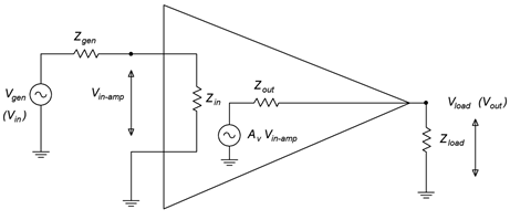
Figure \(\PageIndex{1}\)
2. Determine the load voltage for the model of Figure \(\PageIndex{1}\) given \(V_{gen}\) = 8 mV, \(Z_{gen}\) = 1 k \(\Omega\), \(Z_{in}\) = 6 k\(\Omega\), \(Z_{out}\) = 500 \(\Omega\), \(Z_{load}\) = 2 k \(\Omega\) and \(A_v\) = 100.
3. If the circuit of Problem 1 has a compliance of 2 volts, will the output clip? What if the input is increased to 100 mV?
4. If the circuit of Problem 2 has a compliance of 5 volts, will the output clip? What if the input is increased to 200 mV?
5. If an amplifier has \(A_v\) = 25, \(V_{in}\) = 20 mV and there is no appreciable loading, determine the output signal-to-noise ratio if the amplifier generates an output noise voltage of 10 \(\mu\)V.
6. Determine which waveforms from Figures \(\PageIndex{2}\) through \(\PageIndex{6}\) exhibit halfwave symmetry.
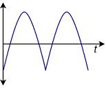
Figure \(\PageIndex{2}\)
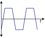
Figure \(\PageIndex{3}\)
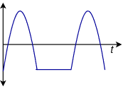
Figure \(\PageIndex{4}\)
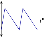
Figure \(\PageIndex{5}\)
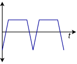
Figure \(\PageIndex{6}\)
7. Determine the Miller equivalent resistances for the circuit of Figure \(\PageIndex{7}\) if \(A_v\) = −20 and \(R\) = 60 k\(\Omega\).
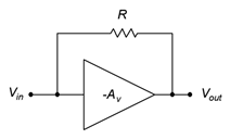
Figure \(\PageIndex{7}\)
8. Determine the Miller equivalent capacitances for the circuit of Figure \(\PageIndex{8}\) assuming \(A_v\) = −30 and \(C\) = 200 pF.
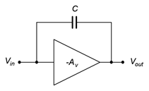
Figure \(\PageIndex{8}\)
6.7.2: Challenge Problems
9. If the circuit of Problem 1 has a compliance of 20 volts, how large can the input signal be before the load voltage is clipped?
10. If the circuit of Problem 2 has a compliance of 10 volts, how large can the input signal be before the load voltage is clipped?
11. Using Figure \(\PageIndex{7}\) as a guide and assuming that \(R\) = 100 k\(\Omega\), how large would the gain have to be such that the input equivalent resistance is 4 k\(\Omega\)?
12. Using Figure \(\PageIndex{8}\) as a guide and assuming that \(A_v\) = −35, determine a value for \(C\) such that the input equivalent capacitance is 1.2 nF.
6.7.3: Computer Simulation Problems
13. Simulate the circuit of Problem 1 and verify the load voltage.
14. Simulate the circuit of Problem 2 and verify the load voltage.