5.7: Projections
- Page ID
- 10135
Computer screens and printers are two-dimensional display devices. We must somehow convert three-dimensional images to two dimensions in order to display them. This task is done by another kind of matrix operator called a projection.
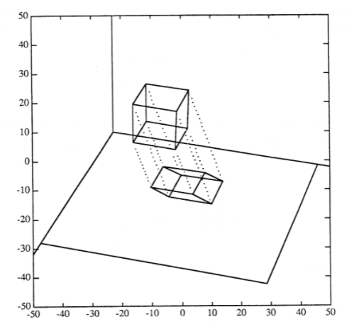
To build a projection, we first choose a projection plane in the three- dimensional space of the object we wish to view. All points of the object are then projected onto the plane. There are many different kinds of projections, corresponding to various geometric rules for mapping points in space onto a plane. We begin with the parallel projection illustrated in Figure 1, wherein the dotted lines between the points and their projections in the plane are all parallel to one another. These dotted lines are called projectors.
Range
The projection plane is called the range of the projection. We will assume for now that the projection plane passes through the origin. If it does not, we may later compose the necessary translations with our projection. Three points, not all in a line, are required to determine a plane. We will take the origin as one of the points and suppose that the other two points are the vectors \(r_1\) and \(r_2\). From these vectors, we form the matrix
\[\mathrm{R}=\left[\mathrm{r}_{1} \mathrm{r}_{2}\right] \nonumber \]
which determines the range of the projection.

Null-Space
To complete the specification of the parallel projection, we must specify the direction of the projectors. The line through the origin in this direction is called the null-space of the projection. Note that any line in the three-dimensional object that is parallel to the null-space will disappear to a point when projected. The null-space may be specified by a vector \(n\) pointing in the direction of the projectors.
Orthogonal Projection
If the null-space is perpendicular to the range, we say that the projection is an orthogonal projection. The matrix operator for orthogonal projection is a function of the range. If we assume that \(R\) is specified in three-dimensional coordinates (not homogeneous!), we have the following definition for the orthogonal projection onto the range of \(R\):
\[\mathrm{P}(\mathrm{R})=\mathrm{R}\left(\mathrm{R}^{T} \mathrm{R}\right)^{-1} \mathrm{R}^{T} \in \mathscr{R}^{3 \times 3} \nonumber \]
In homogeneous coordinates, we embed this 3×3 projection matrix in the general 4×4 transformation:
\[\mathrm{P}_{h}(\mathrm{R})=\left[\begin{array}{ll}
\mathrm{P}(\mathrm{R}) & 0 \\
0^{T} & 1
\end{array}\right] \nonumber \]
Suppose we choose the \(x−y\) plane as our projection plane. Vectors \(r_1\) and \(r_2\) can be any two points in the plane (besides the origin), so let's take
\[\mathrm{r}_{1}=\left[\begin{array}{l}
1 \\
0 \\
0
\end{array}\right], \mathrm{r}_{2}=\left[\begin{array}{l}
1 \\
1 \\
0
\end{array}\right] \nonumber \]
Then the range matrix is
\[\mathrm{R}=\left[\begin{array}{ll}
1 & 1 \\
0 & 1 \\
0 & 0
\end{array}\right] \nonumber \]
The orthogonal projection looking down on the \(x−y\) plane from the z-axis is
\[\begin{align}
\mathrm{P}(\mathrm{R}) &=\left[\begin{array}{ll}
1 & 1 \\
0 & 1 \\
0 & 0
\end{array}\right]\left(\left[\begin{array}{lll}
1 & 0 & 0 \\
1 & 1 & 0
\end{array}\right]\left[\begin{array}{ll}
1 & 1 \\
0 & 1 \\
0 & 0
\end{array}\right]\right)^{-1}\left[\begin{array}{lll}
1 & 0 & 0 \\
1 & 1 & 0
\end{array}\right] \nonumber \\
&=\left[\begin{array}{lll}
1 & 0 & 0 \\
0 & 1 & 0 \\
0 & 0 & 0
\end{array}\right] .
\end{align} \nonumber \]
In homogeneous coordinates,
\[\mathrm{P}_{h}(\mathrm{R})=\left[\begin{array}{llll}
1 & 0 & 0 & 0 \\
0 & 1 & 0 & 0 \\
0 & 0 & 0 & 0 \\
0 & 0 & 0 & 1
\end{array}\right] \nonumber \]
Let the vectors \(\mathrm{r}_{1}=\left[\begin{array}{l}
2 \\
0 \\
0
\end{array}\right]\) and \(\mathrm{r}_{2}=\left[\begin{array}{l}
0 \\
3 \\
0
\end{array}\right]\) specify the range of an orthogonal projection. Find P(R) and P\(_h\)(R). Compare with Example 1 and explain any similarities.
In the chapter on linear algebra you learned that the projection of \(w\) onto \(x\) is given by
\[\mathrm{z}=\frac{(\mathrm{x}, \mathrm{w}) \mathrm{x}}{(\mathrm{x}, \mathrm{x})} \nonumber \]
This is an orthogonal projection of \(w\) onto a line, but it is closely related to the projection into the plane just described. To see the similarity, let's work on the expression for \(z\) a little:
\[\begin{align}
\mathbf{z} &=\frac{\mathrm{x}(\mathrm{x}, \mathrm{w})}{(\mathrm{x}, \mathrm{x})} \nonumber \\
&=\mathrm{x}(\mathrm{x}, \mathrm{x})^{-1}(\mathrm{x}, \mathrm{w}) \nonumber \\
&=\mathrm{x}\left(\mathrm{x}^{T} \mathrm{x}\right)^{-1}\left(\mathrm{x}^{T} \mathrm{w}\right) \nonumber\\
&=\left[\mathrm{x}\left(\mathrm{x}^{T} \mathrm{x}\right)^{-1} \mathrm{x}^{T}\right] \mathrm{w} \nonumber\\
&=\mathrm{P}(\mathrm{x}) \mathrm{w} .
\end{align} \nonumber \]
So we see that it can be written in the same way as the projection onto the plane. The only difference is that the range is now one-dimensional and specified by \(x\) in place of \(R\).
Oblique Projection
More generally, we may have a null-space \(n\) that is not perpendicular to the range R. The projection shown in Figure 1 is an oblique projection. Once again we start with nonhomogeneous coordinates for \(n\) and \(R\) and write the 3×3 oblique projection as
\[\mathrm{E}(\mathrm{R}, \mathrm{n})=\mathrm{R}\left\{\mathrm{R}^{T}[I--P(n)] \mathrm{R}\right\}^{-1} \mathrm{R}^{T}[I--P(n)] \nonumber \]
where
\[\mathrm{P}(\mathrm{n})=\mathrm{n}\left(\mathrm{n}^{T} \mathrm{n}\right)^{-1} \mathrm{n}^{T}=\frac{\mathrm{n} \mathrm{n}^{T}}{\|\mathrm{n}\|^{2}} \nonumber \]
As with the orthogonal projection, we can return to homogeneous coordinates by
\[\mathrm{E}_{h}(\mathrm{R}, \mathrm{n})=\left[\begin{array}{lll}
\mathrm{E}(\mathrm{R} & \mathrm{n}) & 0 \\
\mathrm{O}^{T} & & 1
\end{array}\right] \nonumber \]
Prove and interpret the following properties of paralle1 projections (both orthogonal and oblique):
- P\(^2\) = P; E\(^2\) = E.
- \(PR\)=R; \(ER\)=R.
- \(En\)=0; \(Pn\)=0. (First show that R\(^T\)n=0 when \(n\) is orthogonal to \(R\)).
Display from Projections
Even after we have used a projection, the image points are in three-dimensional homogeneous coordinates. How then do we display them on a two-dimensional display? If we had chosen the \(x−y\) plane as the range of our projection, we could let the output device represent the \(x−y\) plane and ignore the z-coordinate of each point. The z-coordinates of the projected image would all be 0 anyway since the projected points would lie in the \(x−y\) plane. The fourth coordinate of 1 may also be ignored for display. But even if the projection plane is not the \(x−y\) plane, we may perform a rotation to align the two planes and again let the output device represent the \(x−y\) plane.
Perspective Projections
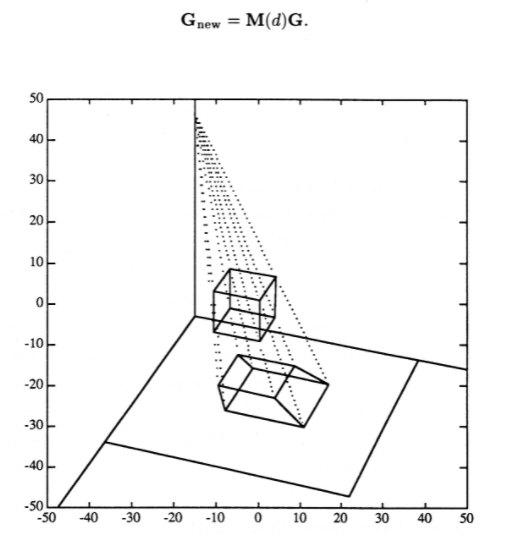
To obtain a perspective projection, we first choose a projection plane as we did for parallel projections. Instead of choosing a null-space parallel to all projectors, we now choose a viewpoint. The projectors all pass through the viewpoint in a perspective projection, as shown in Figure 2. For a viewpoint at \(z=d\) on the z-axis and a projection plane coinciding with the \(x−y\) plane, the three-dimensional homogeneous operator for perspective projection is
\[\mathbf{M}(d)=\left[\begin{array}{llll}
1 & 0 & 0 & 0 \\
0 & 1 & 0 & 0 \\
0 & 0 & 0 & 0 \\
0 & 0 & \frac{-1}{d} & 1
\end{array}\right] \nonumber \]
The first thing you should notice about the perspective projection M(\(d\)) is that it violates the structure given in Equation 2 from "Vector Graphics: Three-Dimensional Homogeneous Coordinates" by having the 4,3 position equal to −\(\frac{1}{d}\) rather than to 0. This means that the fourth coordinates will not remain 1 in the new point matrix
\[\mathrm{G}_{\text {new }}=\mathbf{M}(d) \mathbf{G} \nonumber \]

This situation is interpreted to mean that the new point \((x,y,z,w)\) must be renormalized to \((\frac{x}{w}, \frac{y}{w} \frac{z}{w}1)\) before the operation is considered complete. Renormalization adds another computational step to the image transformation process. This is undesirable, but we are stuck with it if we wish to include perspective projections in our repertoire of transformations. Note that renormalization is a point-by-point process since \(w\) may be different for each point.
How does renormalization affect composition of operators? We might expect that, each time we perform an operation requiring renormalization, we will be forced to stop and do the renormalization before going on with other operations. In this respect we are fortunate: we may put off the renormalization until all transformations are complete and renormalize once just before displaying the image. Thus we are able to compose perspective projections at will with other transformations.
What is the perspective projection matrix for a viewpoint at infinity, M(\(\infty\))? Interpret the result.
Generalization of Projections
“Projection” is a technical term in linear algebra. A square matrix of any size is considered a projection if it obeys the property of Exercise 2(a), P\(^2\)=P. All of our geometric projection matrices have this property. We have considered only three-dimensional spaces with a two-dimensional range and a one-dimensional null-space. In general, the dimensionality of the space may be split in any way between range and null-space. If we reinterpret homogeneous coordinates as four-dimensional space, we have projections with three-dimensional range and one-dimensional null-space, but the perspective projection is actually not quite a projection in the technical sense even though M\(^2(d)\)=M(\(d\)) because perspective projection also includes renormalization.


