The (forward, one-dimensional) discrete Fourier transform (DFT) of an array XX" role="presentation" style="position:relative;" tabindex="0">\(\mathbf{X}\) \(n\) complex numbers is the array XX" role="presentation" style="position:relative;" tabindex="0">\(\mathbf{Y}\) given by
YY" role="presentation" style="position:relative;" tabindex="0">\[\mathbf{Y}[k]=\sum_{l=0}^{n-1}\mathbf{X}[l]\omega _{n}^{lk} \nonumber \]
where \(0\leq k< n\) and \(\omega _n=\text{exp}(-2\pi i/n)\) is a primitive root of unity. Implemented directly, the equation would require Θ(n2)Θ(n2)" role="presentation" style="position:relative;" tabindex="0">\(\Theta (n^2)\) operations; fast Fourier transforms are O(nlogn)O(nlogn)" role="presentation" style="position:relative;" tabindex="0">\(O(n\log n)\) algorithms to compute the same result. The most important FFT (and the one primarily used in FFTW) is known as the “Cooley-Tukey” algorithm, after the two authors who rediscovered and popularized it in 1965, although it had been previously known as early as 1805 by Gauss as well as by later re-inventors. The basic idea behind this FFT is that a DFT of a composite size n=n1n2n=n1n2" role="presentation" style="position:relative;" tabindex="0">\(n=n_1n_2\) can be re-expressed in terms of smaller DFTs of sizes n1n1" role="presentation" style="position:relative;" tabindex="0">\(n_1\) and n1n1" role="presentation" style="position:relative;" tabindex="0">\(n_2\)—essentially, as a two-dimensional DFT of size n1×n2n1×n2" role="presentation" style="position:relative;" tabindex="0">\(n_1\times n_2\) where the output is transposed. The choices of factorizations of n1n1" role="presentation" style="position:relative;" tabindex="0">\(n\)nn" role="presentation" style="position:relative;" tabindex="0">, combined with the many different ways to implement the data re-orderings of the transpositions, have led to numerous implementation strategies for the Cooley-Tukey FFT, with many variants distinguished by their own names. FFTW implements a space of many such variants, as described in Adaptive Composition of FFT Algorithms, but here we derive the basic algorithm, identify its key features, and outline some important historical variations and their relation to FFTW.
The Cooley-Tukey algorithm can be derived as follows. If n1n1" role="presentation" style="position:relative;" tabindex="0">\(n\) can be factored into n=n1n2n=n1n2" role="presentation" style="position:relative;" tabindex="0">\(n=n_1n_2\), the equation can be rewritten by letting \(l=l_1n_2+l_2\) and \(k=k_1+k_2n_1\). We then have:
\[\mathbf{Y}\left [ k_1+k_2n_1\right ]=\sum_{l_2=0}^{n_2-1}\left [ \left ( \sum_{l_1=0}^{n_1-1}\mathbf{X}[l_1n_2+l_2]\omega _{n_1}^{l_1k_1}\right ) \omega _{n}^{l_2k_1}\right ]\omega _{n_2}^{l_2k_2} \nonumber \]
where \(k_{1,2}=0,...n_{1,2}-1\). Thus, the algorithm computes n1n1" role="presentation" style="position:relative;" tabindex="0">\(n_2\) DFTs of size n1n1" role="presentation" style="position:relative;" tabindex="0">n1n1" role="presentation" style="position:relative;" tabindex="0">\(n_1\) (the inner sum), multiplies the result by the so-called twiddle factors \(\omega _{n}^{l_2k_1}\) and finally computes n1n1" role="presentation" style="position:relative;" tabindex="0">\(n_1\) DFTs of size n1n1" role="presentation" style="position:relative;" tabindex="0">n1n1" role="presentation" style="position:relative;" tabindex="0">\(n_2\) n1n1" role="presentation" style="position:relative;" tabindex="0">(the outer sum). This decomposition is then continued recursively. The literature uses the term radix to describe an n1n1" role="presentation" style="position:relative;" tabindex="0">\(n_1\) or n1n1" role="presentation" style="position:relative;" tabindex="0">\(n_2\)n1n1" role="presentation" style="position:relative;" tabindex="0"> that is bounded (often constant); the small DFT of the radix is traditionally called a butterfly.
Many well-known variations are distinguished by the radix alone. A decimation in time (DIT) algorithm uses n1n1" role="presentation" style="position:relative;" tabindex="0">n1n1" role="presentation" style="position:relative;" tabindex="0">\(n_2\) as the radix, while a decimation in frequency (DIF) algorithm uses n1n1" role="presentation" style="position:relative;" tabindex="0">\(n_1\) as the radix. If multiple radices are used, e.g. for nn" role="presentation" style="position:relative;" tabindex="0">n2n2" role="presentation" style="position:relative;" tabindex="0">n1n1" role="presentation" style="position:relative;" tabindex="0">\(n\) composite but not a prime power, the algorithm is called mixed radix. A peculiar blending of radix 2 and 4 is called split radix, which was proposed to minimize the count of arithmetic operations, although it has been superseded in this regard. FFTW implements both DIT and DIF, is mixed-radix with radices that are adapted to the hardware, and often uses much larger radices (e.g. radix 32) than were once common. On the other end of the scale, a “radix” of roughly \(\sqrt{n}\) has been called a four-step FFT algorithm (or six-step, depending on how many transposes one performs); see FFTs and the Memory Hierarchy for some theoretical and practical discussion of this algorithm.
A key difficulty in implementing the Cooley-Tukey FFT is that the n1n1" role="presentation" style="position:relative;" tabindex="0">\(n_1\) dimension corresponds to discontiguous inputs ℓ1ℓ1" role="presentation" style="position:relative;" tabindex="0">n1n1" role="presentation" style="position:relative;" tabindex="0">n1n1" role="presentation" style="position:relative;" tabindex="0">\(l_1\) in \(\mathbf{X}\) but contiguous outputs k1k1" role="presentation" style="position:relative;" tabindex="0">ℓ1ℓ1" role="presentation" style="position:relative;" tabindex="0">n1n1" role="presentation" style="position:relative;" tabindex="0">n1n1" role="presentation" style="position:relative;" tabindex="0">\(k_1\) \(\mathbf{Y}\), and vice-versa for n1n1" role="presentation" style="position:relative;" tabindex="0">n1n1" role="presentation" style="position:relative;" tabindex="0">\(n_2\). This is a matrix transpose for a single decomposition stage, and the composition of all such transpositions is a (mixed-base) digit-reversal permutation (or bit-reversal, for radix 2). The resulting necessity of discontiguous memory access and data re-ordering hinders efficient use of hierarchical memory architectures (e.g., caches), so that the optimal execution order of an FFT for given hardware is non-obvious, and various approaches have been proposed.
n2n2" role="presentation" style="position:relative;" tabindex="0">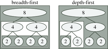
Fig. 10.2.1 Schematic of traditional breadth-first (left) vs. recursive depth-first (right) ordering for radix-2 FFT of size 8: the computations for each nested box are completed before doing anything else in the surrounding box. Breadth-first computation performs all butterflies of a given size at once, while depth-first computation completes one subtransform entirely before moving on to the next (as in the algorithm below).
One ordering distinction is between recursion and iteration. As expressed above, the Cooley-Tukey algorithm could be thought of as defining a tree of smaller and smaller DFTs, as depicted in Fig. 10.2.1; for example, a textbook radix-2 algorithm would divide size nn" role="presentation" style="position:relative;" tabindex="0">n2n2" role="presentation" style="position:relative;" tabindex="0">n1n1" role="presentation" style="position:relative;" tabindex="0">\(n\) into two transforms of size nn" role="presentation" style="position:relative;" tabindex="0">n2n2" role="presentation" style="position:relative;" tabindex="0">n1n1" role="presentation" style="position:relative;" tabindex="0">\(n/2\), which are divided into four transforms of size nn" role="presentation" style="position:relative;" tabindex="0">n2n2" role="presentation" style="position:relative;" tabindex="0">n1n1" role="presentation" style="position:relative;" tabindex="0">\(n/4\), n/4n/4" role="presentation" style="position:relative;" tabindex="0">and so on until a base case is reached (in principle, size 1). This might naturally suggest a recursive implementation in which the tree is traversed “depth-first” as in Fig. 10.2.1 (right) and the algorithm of Pre—one size (n/2n/2" role="presentation" style="position:relative;" tabindex="0">below) nn" role="presentation" style="position:relative;" tabindex="0">n2n2" role="presentation" style="position:relative;" tabindex="0">n1n1" role="presentation" style="position:relative;" tabindex="0">\(n/2\) transform is solved completely before processing the other one, and so on. However, most traditional FFT implementations are non-recursive (with rare exceptions) and traverse the tree “breadth-first” as in Fig. 10.2.1 (left)—in the radix-2 example, they would perform nn" role="presentation" style="position:relative;" tabindex="0">n2n2" role="presentation" style="position:relative;" tabindex="0">n1n1" role="presentation" style="position:relative;" tabindex="0">\(n\) (trivial) size-1 transforms, then n/2n/2" role="presentation" style="position:relative;" tabindex="0">nn" role="presentation" style="position:relative;" tabindex="0">nn" role="presentation" style="position:relative;" tabindex="0">n2n2" role="presentation" style="position:relative;" tabindex="0">n1n1" role="presentation" style="position:relative;" tabindex="0">\(n/2\) combinations into size-2 transforms, then n/4n/4" role="presentation" style="position:relative;" tabindex="0">nn" role="presentation" style="position:relative;" tabindex="0">n2n2" role="presentation" style="position:relative;" tabindex="0">n1n1" role="presentation" style="position:relative;" tabindex="0">\(n/4\) combinations into size-4 transforms, and so on, thus making log2nlog2n" role="presentation" style="position:relative;" tabindex="0">\(\log _2n\) passes over the whole array. In contrast, as we discuss in Adaptive Composition of FFT Algorithms, FFTW employs an explicitly recursive strategy that encompasses both depth-first and breadth-first styles, favoring the former since it has some theoretical and practical advantages as discussed in FFTs and the Memory Hierarchy.
A second ordering distinction lies in how the digit-reversal is performed. The classic approach is a single, separate digit-reversal pass following or preceding the arithmetic computations; this approach is so common and so deeply embedded into FFT lore that many practitioners find it difficult to imagine an FFT without an explicit bit-reversal stage. Although this pass requires only O(n)O(n)" role="presentation" style="position:relative;" tabindex="0">\(O(n)\) time, it can still be non-negligible, especially if the data is out-of-cache; moreover, it neglects the possibility that data reordering during the transform may improve memory locality. Perhaps the oldest alternative is the Stockham auto-sort FFT, which transforms back and forth between two arrays with each butterfly, transposing one digit each time, and was popular to improve contiguity of access for vector computers. Alternatively, an explicitly recursive style, as in FFTW, performs the digit-reversal implicitly at the “leaves” of its computation when operating out-of-place (see section Adaptive Composition of FFT Algorithms). A simple example of this style, which computes in-order output using an out-of-place radix-2 FFT without explicit bit-reversal, is shown in the algorithm of above[corresponding to Fig. 10.2.1 (right)]. To operate in-place with O(n)O(n)" role="presentation" style="position:relative;" tabindex="0">\(O(1)\) scratch storage, one can interleave small matrix transpositions with the butterflies and a related strategy in FFTW is briefly described by Adaptive Composition of FFT Algorithms.
Finally, we should mention that there are many FFTs entirely distinct from Cooley-Tukey. Three notable such algorithms are the prime-factor algorithm for \(\text{gcd}(n_1,n_2)=1\) along with Rader's and Bluestein's algorithms for prime nn" role="presentation" style="position:relative;" tabindex="0">n2n2" role="presentation" style="position:relative;" tabindex="0">n1n1" role="presentation" style="position:relative;" tabindex="0">\(n\). FFTW implements the first two in its codelet generator for hard-coded nn" role="presentation" style="position:relative;" tabindex="0">n2n2" role="presentation" style="position:relative;" tabindex="0">n1n1" role="presentation" style="position:relative;" tabindex="0">\(n\) Generating Small FFT Kernels and the latter two for general prime nn" role="presentation" style="position:relative;" tabindex="0">n2n2" role="presentation" style="position:relative;" tabindex="0">n1n1" role="presentation" style="position:relative;" tabindex="0">\(n\) (sections Adaptive Composition of FFT Algorithms and Goals and Background of the FFTW Project). There is also the Winograd FFT which minimizes the number of multiplications at the expense of a large number of additions; this trade-off is not beneficial on current processors that have specialized hardware multipliers.
nn" role="presentation" style="position:relative;" tabindex="0">Contributor

