
2.4: Additional Useful Functions and Laplace Transforms - Step, Sine, Cosine, and Definite Integral
- Page ID
- 7631

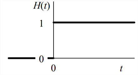
We shall describe and transform several different useful mathematical functions. A common feature of most of these functions is that they are defined to have non-zero values only for positive time, i.e., they are zero before \(t\) = 0. The fundamental function of this type is the basic Heaviside unit-step function (after English electrical engineer, physicist, and applied mathematician Oliver Heaviside, 1850-1925) shown in Figure \(\PageIndex{1}\):
\[H(t)=\left\{\begin{array}{ll}
0 & \text { for } t<0 \\
1 & \text { for } t>0
\end{array}\right.\label{eqn:2.26} \]
\(H(t)\) is dimensionless, and it is undefined mathematically at the discontinuity at \(t = 0\). If we wish to write an equation for a physical input quantity that is applied quickly and remains constant thereafter, we can use \(H(t)\) to represent it approximately; for example, a “step” force \(f_x(t)\) can be described with the equation
\[f_{x}(t)=F \times H(t) \equiv F H(t)\nonumber \]
where \(F\) is the dimensional force magnitude. For many physical input quantities, a step function is an idealized approximation; such a quantity increases quickly but continuously, not as a discontinuous pure step, from zero to a constant value. [The notation \(H(t)\) used here for the unit-step function is common but not standard; in fact, there is no standard symbol in engineering literature.]
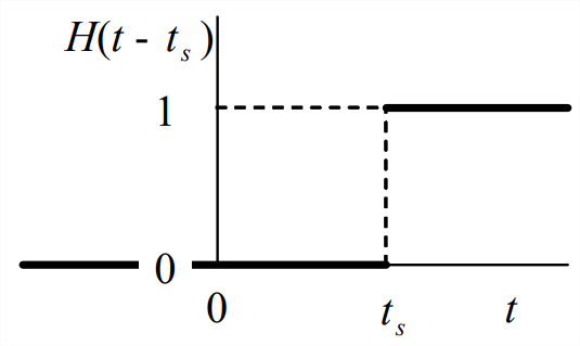
A more general unit-step function describes a step that occurs at some time different than the instant defined to be \(t\) = 0. This function shown in Figure \(\PageIndex{2}\) is:
\[H\left(t-t_{s}\right)=\left\{\begin{array}{ll}
0 & \text { for } t<t_{s} \\
1 & \text { for } t>t_{s}
\end{array}\right.\label{eqn:2.27} \]
If the time of discontinuity is \(t_s = 0\), then this more general function becomes the basic function of Equation \(\ref{eqn:2.26}\). The Laplace transform of \(H\left(t-t_{s}\right)\) is
\[L\left[H\left(t-t_{s}\right)\right]=\int_{t=0}^{t=\infty} e^{-s t} H\left(t-t_{s}\right) d t=\int_{t=t_{s}}^{t=\infty} e^{-s t} d t=\frac{1}{-s} \int_{t-t_{s}}^{t=\infty} d\left(e^{-s t}\right)=-\frac{1}{s}\left(e^{-s \times \infty}-e^{-s t_{s}}\right) \nonumber \]
\[L\left[H\left(t-t_{s}\right)\right]=\frac{e^{-s t_{s}}}{s}\label{eqn:2.28} \]
Note, in particular, the version of Equation \(\ref{eqn:2.28}\) for the basic unit-step function with \(t_s\) = 0:
\[L[H(t)]=\frac{1}{s}\label{eqn:2.29} \]
We will frequently use sine and cosine functions of time with circular frequency \(\omega\), the functions being non-zero only for positive time, \(t\) \(\geq\) 0. Using precise notation, such a sine function, for example, should be denoted \(H(t) \times \sin \omega t\); however, with few exceptions, we will consider mostly \(t\) \(\geq\) 0, so we can almost always omit the “\(H(t) \times\)” part of the equation, with the implicit understanding that the analysis applies only for \(t\) \(\geq\) 0.
Next we derive the Laplace transform of the sine function by expressing the sine in terms of complex exponential functions (homework Problem 2.1) and using the basic forward transform of Equation \(\ref{eqn:2.26}\):
\[L[\sin \omega t]=L\left[\frac{e^{j \omega t}-e^{-j \omega t}}{2 j}\right]=\frac{1}{2 j}\left(\frac{1}{s-j \omega}-\frac{1}{s+j \omega}\right)=\frac{1}{2 j}\left(\frac{s+j \omega-(s-j \omega)}{(s-j \omega)(s+j \omega)}\right) \nonumber \]
\[L[\sin \omega t]=\frac{1}{2 j}\left(\frac{2 j \omega}{s^{2}+\omega^{2}}\right)=\frac{\omega}{s^{2}+\omega^{2}}\label{eqn:2.30} \]
Using a similar process, you can derive (homework Problem 2.10) the following Laplace transform of the cosine function:
\[L[\cos \omega t]=\frac{s}{s^{2}+\omega^{2}}\label{eqn:2.31} \]
Another useful Laplace transform is that of a definite integral. Suppose that a physically realistic function \(f(t)\) has Laplace transform \(F(s)=L[f(t)]\), and that we need the transform of the definite integral \(\int_{\tau=-\infty}^{\tau=t \geq 0} f(\tau) d \tau\). Note the lower limit of \(\tau=-\infty\); we will usually consider \(f(t)\) only for \(t\) \(\geq\) 0, but occasionally the integral of \(f(t)\) over previous time, \(t\) < 0, is also needed. The general transform, which is derived in Appendix A, Section A-3, is:
\[L\left[\int_{\tau=-\infty}^{\tau=t \geq 0} f(\tau) d \tau\right]=\frac{1}{s} F(s)+\frac{1}{s} \int_{\tau=-\infty}^{\tau=0} f(\tau) d \tau\label{eqn:2.32} \]
For most applications, we will have \(f(t)\) = 0 for \(t\) < 0, for which the simpler transform is:
\[L\left[\int_{\tau=0}^{\tau=t \geq 0} f(\tau) d \tau\right]=\frac{1}{s} F(s)\label{eqn:2.33} \]
If we regard the integral of \(f(t)\) as being the first “negative” derivative (antiderivative), then we see that transform Equation \(\ref{eqn:2.32}\) is logically consistent with transform Equation 2.2.9 for a “positive” derivative, with respect to both power of \(s\) and the initial value term.