3.7: More Examples of Damped Mechanical Systems

Last updated
Save as PDF

Page ID: 7961

\( \newcommand{\vecs}[1]{\overset { \scriptstyle \rightharpoonup} {\mathbf{#1}} } \) \( \newcommand{\vecd}[1]{\overset{-\!-\!\rightharpoonup}{\vphantom{a}\smash {#1}}} \)\(\newcommand{\id}{\mathrm{id}}\) \( \newcommand{\Span}{\mathrm{span}}\) \( \newcommand{\kernel}{\mathrm{null}\,}\) \( \newcommand{\range}{\mathrm{range}\,}\) \( \newcommand{\RealPart}{\mathrm{Re}}\) \( \newcommand{\ImaginaryPart}{\mathrm{Im}}\) \( \newcommand{\Argument}{\mathrm{Arg}}\) \( \newcommand{\norm}[1]{\| #1 \|}\) \( \newcommand{\inner}[2]{\langle #1, #2 \rangle}\) \( \newcommand{\Span}{\mathrm{span}}\) \(\newcommand{\id}{\mathrm{id}}\) \( \newcommand{\Span}{\mathrm{span}}\) \( \newcommand{\kernel}{\mathrm{null}\,}\) \( \newcommand{\range}{\mathrm{range}\,}\) \( \newcommand{\RealPart}{\mathrm{Re}}\) \( \newcommand{\ImaginaryPart}{\mathrm{Im}}\) \( \newcommand{\Argument}{\mathrm{Arg}}\) \( \newcommand{\norm}[1]{\| #1 \|}\) \( \newcommand{\inner}[2]{\langle #1, #2 \rangle}\) \( \newcommand{\Span}{\mathrm{span}}\)\(\newcommand{\AA}{\unicode[.8,0]{x212B}}\)

Let us consider next some combinations of dashpots with springs and masses. In each case, we will draw the physical device, draw appropriate free-body diagrams, and then derive the equations of motion. Force \(f_x(t)\) is considered to be an independent input quantity in all of these examples.

Example \(\PageIndex{1}\)

Newton’s 2nd law for translation of the mass: \(m \ddot{x}=f_{x}(t)-c \dot{x}-k x\)

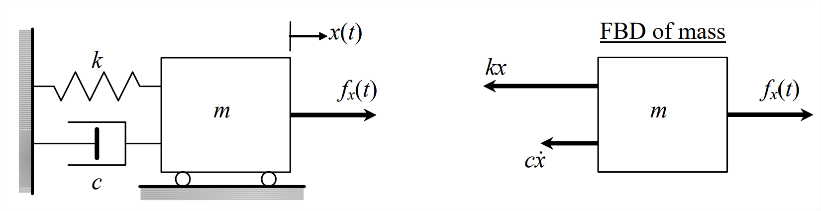
Figure \(\PageIndex{1}\): Mass-damper-spring system

Solution

\[\Rightarrow \quad \text { ODE }: \quad m \ddot{x}+c \dot{x}+k x=f_{x}(t)\label{eqn:3.20} \]

Example \(\PageIndex{2}\)

This combination is very similar to the mass-damper-spring system, except the inertial force of the mass (now considered just a rigid link) is assumed to be negligible.

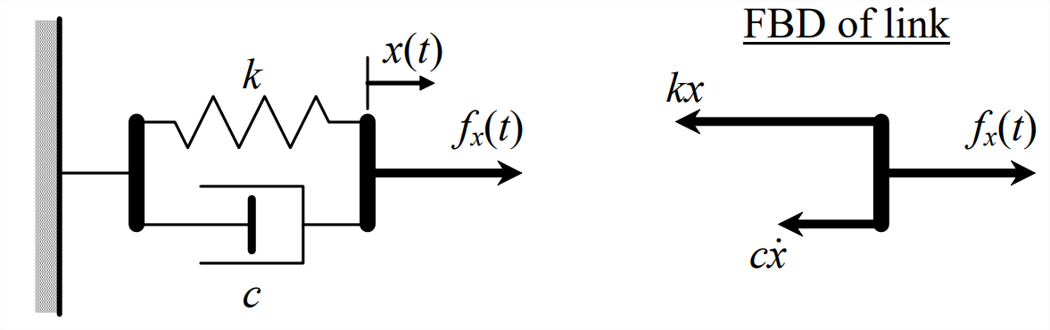
Figure \(\PageIndex{2}\): Parallel damper-spring system

Solution

Newton’s 2^nd law for translation of the link: \(m \ddot{x} \cong 0=f_{x}(t)-c \dot{x}-k x\)

\[\Rightarrow \text { ODE : } c \dot{x}+k x=f_{x}(t)\label{eqn:3.21} \]

Note that Equation \(\ref{eqn:3.21}\) is a typical 1^st order LTI ODE, but now the unknown quantity is translation (position) \(x(t)\) of the rigid link.

Example \(\PageIndex{3}\)

For the examples above, it is not necessary to draw separate FBDs of the spring and of the dashpot’s piston and cylinder. However, it is necessary to draw separate FBDs for systems such as that of Figure \(\PageIndex{3}\), where dashpot and spring are arranged in series, not in parallel, and, for variety and generality, the inertial forces of the dashpot’s piston and cylinder are considered to be significant, not negligible. Take notice of the component interaction forces \(f_c\) and \(f_k\); note especially that piston-cylinder interaction force \(f_c\) is shown as an equal and opposite pair, as required by Newton’s 3^rd law.

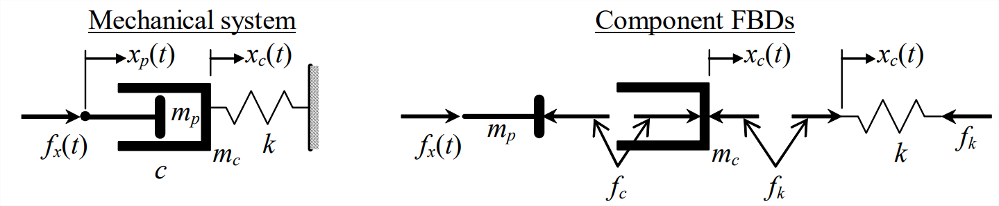
Figure \(\PageIndex{3}\): Example series mass-dashpot-spring

Newton’s 2^nd law for translation of the dashpot piston: \(m_{p} \ddot{x}_{p}=f_{x}(t)-f_{c}\)

Newton’s 2^nd law for translation of the dashpot cylinder: \(m_{c} \ddot{x}_{c}=f_{c}-f_{k}\)

Damper law: \(f_{c}=c\left(\dot{x}_{p}-\dot{x}_{c}\right)\)

Spring law: \(f_{k}=k x_{c}\)

Solution

Combining equations of motion and damper/spring laws gives:

\[m_{p} \ddot{x}_{p}+c \dot{x}_{p}-c \dot{x}_{c}=f_{x}(t)\label{eqn:3.22a} \]

\[m_{c} \ddot{x}_{c}-c \dot{x}_{p}+c \dot{x}_{c}+k x_{c}=0\label{eqn:3.22b} \]

Equations \(\ref{eqn:3.22a}\) and \(\ref{eqn:3.22b}\) are a pair of coupled 2^nd order ODEs in the two dependent variables \(x_p(t)\) and \(x_c(t)\). Thus, the system of Figure \(\PageIndex{3}\) is a 4^th order system. The dynamic response of a particular class of 4^th order systems is discussed Chapter 12. However, this book does not address the dynamic response of general 4^th order and higher-order systems; that is a subject of more advanced textbooks such as Ogata, 1998, Chapter 10.

Example \(\PageIndex{4}\)

For both of the series damper-spring combinations in Figure \(\PageIndex{4}\), we specify the known input quantity to be translation \(x_i(t)\), which is produced by an idealized motor that is capable of dictating a commanded displacement regardless of the force required. The output quantity in each case is translation \(x_0(t)\). The damper and spring masses are assumed here to be negligible, which cannot be valid for all practical circumstances; therefore, these are idealized, not real, mechanical systems. But these idealized systems are worth studying because they have significant dynamic characteristics that will be the subjects of subsequent parts of this book.

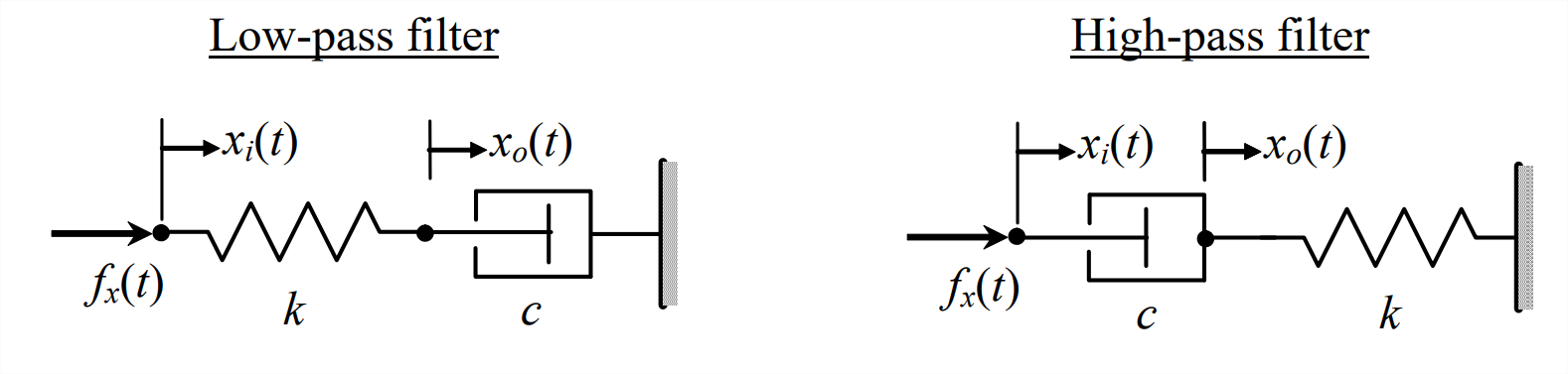
Figure \(\PageIndex{4}\): Series damper-spring idealized mechanical filters

Solution

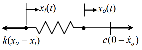
Figure \(\PageIndex{5}\): FBD of series damper-spring idealized mechanical filters

The governing ODE for the low-pass filter, with spring and damper masses idealized to be negligible, is derived easily from the FBD at right of the series combination consisting of the spring and the damper piston: \(k\left(x_{o}-x_{i}\right)=c\left(0-\dot{x}_{o}\right)\). Therefore the ODE for the low-pass filter is

\[\dot{x}_{o}+\frac{1}{\tau_{1}} x_{o}=\frac{1}{\tau_{1}} x_{i}(t), \quad \tau_{1} \equiv \frac{c}{k}\label{eqn:3.23} \]

The mathematical derivation and description of low-pass-filter characteristics will follow in later chapters, but it is appropriate here to describe the practical nature of the low-pass filter with use of the low-pass filter drawing in Figure \(\PageIndex{4}\) and physical intuition. Imagine that the input translation \(x_i(t)\) is a steady oscillation at a fixed frequency. If that frequency is very low, so that translational velocity is low, then the damper resisting force \(c \dot{x}_{o}\) will be very small and, consequently, both the spring and the damper piston will move slowly back and forth in unison by about the same distance as the input translation, \(x_{o}(t) \approx x_{i}(t)\). On the other hand, if the frequency of oscillation is very high, then the damper resisting force \(c \dot{x}_{o}\) will be great, so the input oscillatory translation \(x_i(t)\) will compress and stretch the spring but the damper piston will act almost like a rigid wall, i.e., \(x_{o}(t) \approx 0\). For frequencies of oscillation between very low and very high, our intuition suggests that the output motion amplitude [the maximum of oscillatory \(x_{o}(t)\)] will be between the two extremes of the input motion amplitude and zero motion. The low-pass filter is so named because it “passes” through, without much alteration, low-frequency inputs, but it “blocks” high-frequency inputs.

Derivation of the governing ODE for the damper-spring high-pass filter is left for homework Problem 3.7. The result is:

\[\dot{x}_{o}+\frac{1}{\tau_{1}} x_{o}=\dot{x}_{i}(t), \quad \tau_{1} \equiv \frac{c}{k}\label{eqn:3.24} \]

As is done above for the damper-spring low-pass-filter, it is appropriate to describe the practical nature of the high-pass filter with use of the high-pass filter drawing in Figure \(\PageIndex{4}\) and physical intuition. Imagine that the input translation \(x_i(t)\) is a steady oscillation at a fixed frequency. If that frequency is very low, so that translational velocity is low, then the damper resisting force \(c\left(\dot{x}_{i}-\dot{x}_{o}\right)\) will be very small; consequently, the damper piston will move slowly back and forth within the cylinder by about the same distance as the input translation; but very little force will be imposed upon the cylinder and spring, so the spring will be deformed hardly at all, \(x_{o}(t) \approx 0\). On the other hand, if the frequency of oscillation is very high, then the damper resisting force \(c\left(\dot{x}_{i}-\dot{x}_{o}\right)\) will be great, so the piston and cylinder will appear to become a single rigid body, and most of the input translation will be transmitted through the damper, \(x_{o}(t) \approx x_{i}(t)\), to compress and stretch the spring. For frequencies of oscillation between very low and very high, our intuition suggests that the output motion amplitude will be between the two extremes of zero motion and the input motion amplitude. The high-pass filter is so named because it “blocks” low-frequency inputs, but it “passes” through, without much alteration, high-frequency inputs.

The damper-spring high-pass filter system is said to have right-hand-side (RHS) dynamics due to the explicit derivative of the input translation, \(\dot{x}_{i}\), on the RHS of ODE Equation \(\ref{eqn:3.24}\). Therefore, Equation \(\ref{eqn:3.24}\) does not have the standard stable 1^st order form of Equation 3.4.8, \(\dot{x}+\left(1 / \tau_{1}\right) x=b u(t)\), with the input \(u(t)\) on the RHS, but none of its derivatives. For standard forms such as Equation 3.4.8, many readily available mathematical response solutions exist, e.g., step response Equation 3.4.9. But that is not the case for non-standard forms, so the non-standard character might be considered inconvenient. However, there is a process at converts non-standard ODE Equation \(\ref{eqn:3.24}\) into standard form¹. We define the difference variable \(x_d(t)\):

\[x_{d}(t)=x_{o}(t)-x_{i}(t)\label{eqn:3.25} \]

Differentiating Equation \(\ref{eqn:3.25}\) and substituting the result into Equation \(\ref{eqn:3.24}\) leads to the following standard-form ODE for \(x_d(t)\) plus the auxiliary equation required to retrieve the desired output \(x_0(t)\) from solution \(x_d(t)\) of the ODE:

\[\dot{x}_{d}+\frac{1}{\tau_{1}} x_{d}=-\frac{1}{\tau_{1}} x_{i}(t), \quad x_{o}(t)=x_{d}(t)+x_{i}(t)\label{eqn:3.26} \]

¹The process shown here for a 1^st order ODE is the simplest form of a more general process that can be applied to system ODEs of any order having RHS dynamics; see the textbook by Brogan, 1974, pages 174- 177.