4.4: Period, Frequency, and Phase of Periodic Signals

Let us consider more generally the temporal quantities of periodic signals, represented in our applications by sinusoids. Period \(T_p\) is normally measured in seconds per cycle, so the cyclic frequency \(f\) in cycles per second is the inverse of period, \(f=1 / T_{p}\). Also, the period is related to the circular frequency \(\omega\) by \(\omega T_{p}=2 \pi\) radians, so that

\[\text { circular frequency } \omega=\frac{2 \pi}{T_{p}} \equiv 2 \pi f \frac{\mathrm{rad}}{\mathrm{sec}}, \text { and cyclicfrequency } f=\frac{\omega}{2 \pi} \mathrm{Hz}\left(\frac{\text { cycles }}{\mathrm{sec}}\right)\label{eqn:4.16} \]

These relationships between period and frequency are worth understanding completely and even memorizing, as we use them a great deal in system dynamics.

It is important also to understand how FRF phase is manifested in time history plots of input and output. This discussion is general, applicable for any LTI system. Suppose that there are plotted on the same graph steady-state sinusoidal time histories of both the input \(u(t)\) and the output \(x(t)\), as in Figure \(\PageIndex{1}\) on the next page. We want to calculate the FRF phase from measurements on the time-history plots. First, find the nearest positive \(x(t)\) crest to the left of a reference positive \(u(t)\) crest, as shown on Figure \(\PageIndex{1}\). Measure the positive time interval \(T_{l e a d}\) in seconds that \(x(t)\) leads \(u(t)\). (Note that you can measure \(T_{l e a d}\) also by comparing troughs or positive-going or negative-going zeros, as shown on Figure \(\PageIndex{1}\).)

Figure \(\PageIndex{1}\): Frequency response phase measurement from time-history graphs

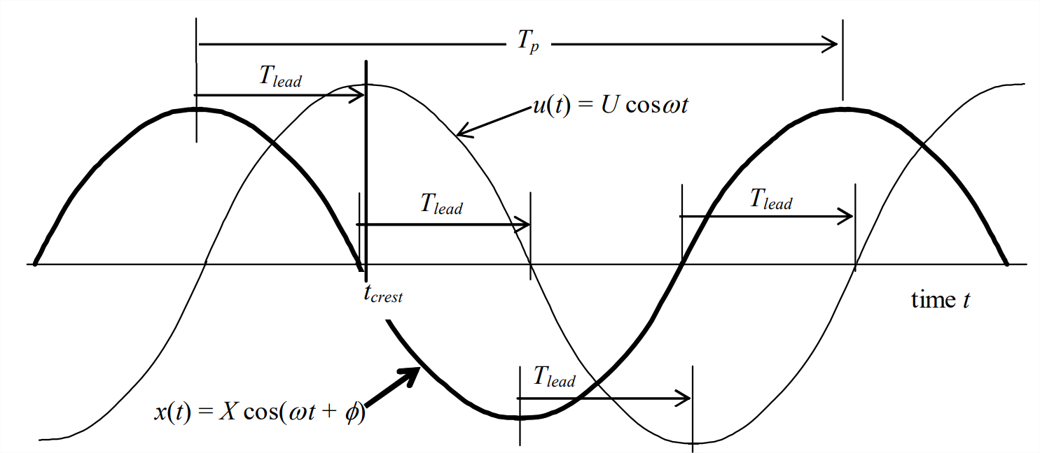
Now, referring to the positive crests, let us denote as \(t_{\text {crest}}\) the instant corresponding to a positive crest of input \(u(t)\). Then we see from the drawing that

\[\cos \omega t_{c r e s t}=+1 \quad \Rightarrow \quad \omega t_{c r e s t}=2 \pi n, \text { where } n \text { is some integer } \nonumber \]

\[\cos \left(\omega\left[t_{\text {crest}}-T_{\text {lead}}\right]+\phi\right)=+1 \quad \Rightarrow \quad \omega\left[t_{\text {crest}}-T_{\text {lead}}\right]+\phi=2 \pi n \nonumber \]

Comparing these two equations shows that \(\omega\left[-T_{l e a d}\right]+\phi=0\), which gives the basic equation for phase angle (defined positive as a lead, negative as a lag):

\[\phi=\omega T_{\text {lead}}=\frac{2 \pi}{T_{p}} T_{\text {lead}}=2 \pi \frac{T_{\text {lead}}}{T_{p}} \operatorname{rad} \times \frac{360 \mathrm{deg}}{2 \pi \mathrm{rad}}=360 \times \frac{T_{\text {lead}}}{T_{p}} \mathrm{deg}\label{eqn:4.17a} \]

where \(T_{p}(=2 \pi / \omega=1 / f)\) is the period of the input and the steady-state output, as shown on Figure \(\PageIndex{1}\).

If you choose to select the nearest positive \(x(t)\) crest to the right of a reference \(u(t)\) crest, then you are finding time lag \(T_{l a g}\), which is a negative lead. In this case, you can find the phase angle, with the correct sign, from

\[\phi=-\omega T_{l a g}=-360 \times \frac{T_{l a g}}{T_{p}} \operatorname{deg}\label{eqn:4.17b} \]

Equations \(\ref{eqn:4.17a}\) and \(\ref{eqn:4.17b}\) give \(\phi\) in the range 0° \(\leq\) \(\phi\) < 360°, which is correct but not common. It is not common because the four-quadrant arctangent is conventionally expressed (in MATLAB, for example) in the range −180° \(\leq\) \(\phi\) < +180°. Therefore, if you measure and calculate by the procedure above a phase \(\phi\) \(\geq\) +180°, then it is conventional to replace that \(\phi\) with (\(\phi\) − 360°). For example, if you were to measure and calculate the phase \(\phi\) = 262°, then it would be conventional to express it as a phase lag, φ = (262° − 360°) = −98°, rather than a phase lead of 262°.