5.2: Passive Components - Resistor, Capacitor, Inductor

We denote the electrical potential, the voltage in volts (V) SI units, at a point in a circuit as \(e(t)\), and the flow of positively charged particles, the electrical current in amps (A) SI units, as \(i(t)\). These two electrical quantities are the principal variables that will appear in derivations of the ODEs describing the dynamic behavior of circuits.

Figure \(\PageIndex{1}\): Resistor in a simple circuit

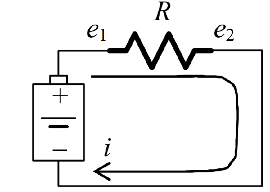
The circuit drawn in Figure \(\PageIndex{1}\) depicts an ideal linear resistor, with resistance \(R\) ohms (usually denoted by the upper-case omega, \(\text{\omega\)\)) in SI units. The voltage difference \(e_{1}-e_{2}\) between the positive and negative terminals of a battery causes current \(i\) to flow through the resistor. The material of the resistor is an electrical conductor, but a poor conductor that provides much more resistance to current flow than a good conductor such as copper wire. This resistance converts part of the electrical energy into heat energy, causing the resistor’s temperature to rise slightly. For a standard, commercially produced resistor, the relationship between \(e_{1}-e_{2}\) and \(i\) is linear, with resistance \(R\) defined as the constant of proportionality (Halliday and Resnick, 1960, Sections 31-2 and 31-3). This relationship is known as Ohm’s law (after German physicist Georg Simon Ohm, 1787-1854), and it is usually expressed in one of the following two forms:

\[e_{1}-e_{2}=i R \Rightarrow i=\frac{e_{1}-e_{2}}{R}\label{eqn:5.1} \]

Equation \(\ref{eqn:5.1}\) applies at each instant, even if the voltages and the current are varying with time.

Note from Ohm’s law the unit equivalence Ω = V/A; this relation giving the ohm in terms of the volt and the amp is useful for establishing correct units in calculations. Suppose, for example, that a 10-volt difference is imposed across a 5 kΩ resistor, typical numbers for instrumentation circuits. Then, from Equation \(\ref{eqn:5.1}\), the current through the resistor is

\[i=\frac{10 \mathrm{V}}{5 \times 10^{3} \mathrm{V} / \mathrm{A}}=2 \mathrm{e}-3 \mathrm{A} \equiv 2 \mathrm{mA}. \nonumber \]

The following two examples serve to introduce a fundamental physical principle for electrical circuits, Kirchhoff’s current law (abbreviated “KCL”, after German physicist Gustav Robert Kirchhoff, 1824-1887), and to illustrate applications of KCL.

Example \(\PageIndex{1}\)

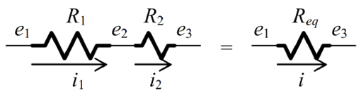
Given resistors \(R_1\) and \(R_2\) arranged in series, as in the figure below, find the equivalent single resistance \(R_{eq}\).

Figure \(\PageIndex{2}\)

Solution

From the figure and Equation \(\ref{eqn:5.1}\),

\[i_{1}=\frac{e_{1}-e_{2}}{R_{1}}, i_{2}=\frac{e_{2}-e_{3}}{R_{2}}, i=\frac{e_{1}-e_{3}}{R_{e q}} \nonumber \]

The form of KCL relevant to this situation is: the quantity of current is continuous in a series arrangement, so that \(i_{1}=i_{2} \equiv i\). [This continuity condition for electrical current is directly analogous to the continuity condition for an incompressible fluid: the volume flow rate (average velocity \(\times\) cross-sectional area) remains constant at all points along a flow tube or channel.] The total voltage change is the sum of the individual changes,

\[e_{1}-e_{3}=\left(e_{1}-e_{2}\right)+\left(e_{2}-e_{3}\right)=i_{1} R_{1}+i_{2} R_{2}=i\left(R_{1}+R_{2}\right) \nonumber \]

\[\Rightarrow \quad i=\frac{e_{1}-e_{3}}{R_{1}+R_{2}} \Rightarrow R_{e q}=R_{1}+R_{2} \nonumber \]

The resistance of a series combination of resistors is the sum of the individual resistances.

Example \(\PageIndex{2}\)

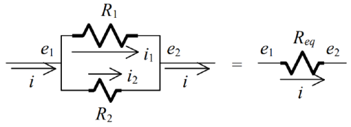
Given resistors \(R_1\) and \(R_2\) arranged in parallel, as in the figure below, find the equivalent single resistance \(R_{eq}\).

Figure \(\PageIndex{3}\)

Solution

In this case, there are circuit junctions on both sides of the parallel resistors. The more general KCL applicable here is: the quantity of current leaving a junction equals the quantity of current entering the junction, so that \(i_{1}+i_{2}=i\). The voltage difference is the same across each of the parallel resistors, so KCL in terms of voltage differences is

\[\frac{e_{1}-e_{2}}{R_{1}}+\frac{e_{1}-e_{2}}{R_{2}}=\frac{e_{1}-e_{2}}{R_{e q}} \Rightarrow \frac{1}{R_{1}}+\frac{1}{R_{2}}=\frac{1}{R_{e q}}=\frac{R_{1}+R_{2}}{R_{1} R_{2}} \Rightarrow R_{e q}=\frac{R_{1} R_{2}}{R_{1}+R_{2}} \nonumber \]

The equivalent (effective) resistance is less than the smaller of the two parallel resistances.

Figure \(\PageIndex{4}\): Capacitor in a simple circuit

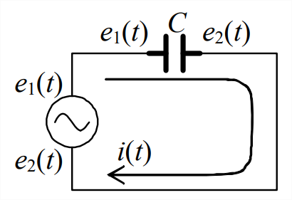
The circuit drawn in Figure \(\PageIndex{4}\) depicts a linear capacitor, with capacitance \(C\) farad (F) in SI units. A voltage generator produces the possibly time-varying voltage difference \(e_{1}-e_{2}\) across the capacitor. The graphical symbol representing the capacitor depicts two plates separated by a dielectric (insulating) material. If there is a voltage difference between the plates of such a component, a positive electrical charge +\(q\) coulombs (SI unit) appears on one plate, and a negative electrical charge −\(q\) coulombs appears on the other plate (Halliday and Resnick, 1960, Section 30-2). The quantity of charge \(q\) is proportional to the voltage difference, with capacitance \(C\) defined as the constant of proportionality:

\[q=C\left(e_{1}-e_{2}\right)\label{eqn:5.2} \]

If the voltage difference is constant, then the charge on the plates remains constant, so that there is no flow of charged particles, i.e., no current, which is the variation with time of the charge: \(i(t)=\frac{d q}{d t}\). However, if the voltage varies with time, then current flows through the circuit in proportion with the derivative of the voltage difference:

\[i(t)=\frac{d q}{d t}=C \frac{d\left(e_{1}-e_{2}\right)}{d t}=C\left(\dot{e}_{1}-\dot{e}_{2}\right)\label{eqn:5.3} \]

Conversely, the voltage difference across the capacitor can be expressed in terms of the current by integrating Equation \(\ref{eqn:5.3}\) from initial time \(t_0\) (when ICs are assumed to be known) to arbitrary time \(t>t_{0}\) :

\[\int_{\tau=t_{0}}^{\tau=t} i(\tau) d \tau=C \int_{\tau=t_{0}}^{\tau=t} \frac{d\left(e_{1}-e_{2}\right)}{d \tau} d \tau=C\left[\left.\left(e_{1}-e_{2}\right)\right|_{t}-\left.\left(e_{1}-e_{2}\right)\right|_{t_{0}}\right] \nonumber \]

\[\Rightarrow e_{1}(t)-e_{2}(t)=e_{1}\left(t_{0}\right)-e_{2}\left(t_{0}\right)+\frac{1}{C} \int_{\tau=t_{0}}^{\tau=t} i(\tau) d \tau\label{eqn:5.4} \]

Note from Equation \(\ref{eqn:5.3}\) the unit equivalence \(A=F \times \frac{V}{s } \Rightarrow F=\frac{A s }{V}\); this relation for the farad in terms of the amp, the volt, and the second is useful for clarifying units in calculations. Suppose, for example, that an instrumentation circuit contains a capacitor with \(C\) = 0.25 \(\mu\)F = 0.25e−6 F, a typical value. If, at a particular instant, the voltage across the capacitor is changing at the rate 6 000 V/s, then the current through the capacitor is, from Equation \(\ref{eqn:5.3}\), \(i=\left(0.25 \times 10^{-6} \frac{\mathrm{A}-\mathrm{sec}}{\mathrm{V}}\right) \times\left(6 \times 10^{3} \frac{\mathrm{V}}{\mathrm{sec}}\right)=1.5 \times 10^{-3} \mathrm{A} \equiv 1.5 \mathrm{mA}\).

Example \(\PageIndex{3}\) - 1^st order, \(RC\) low-pass filter

This is a circuit containing both a resistor and a capacitor. The input voltage signal produced by some source is denoted \(e_{i}(t)\), and the output, filtered signal is denoted \(e_{o}(t)\). Figure \(\PageIndex{5}\) depicts this filter graphically in both the simple closed-circuit form on

Figure \(\PageIndex{5}\): \(RC\) low-pass filter circuit

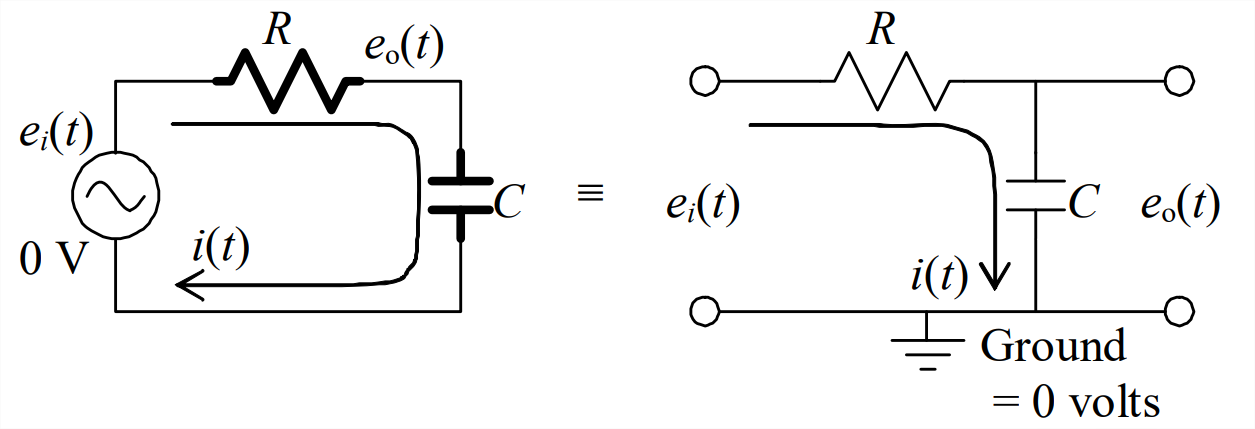
the left, and the more modern form on the right, in which the common ground (reference) potential is denoted by a special symbol and is assigned the value zero volts, to which all other circuit voltages are referenced. The input and output terminals are denoted by small circles. Note, in particular, that the output terminals are isolated away from the current-carrying portion of the circuit; this represents the realistic situation in which the filter output voltage is the input to some other circuit that has a very high input resistance, thereby essentially preventing any input current. This downstream circuit could be some measuring instrument (oscilloscope, voltmeter, etc.), or another stage of a larger circuit of which the \(RC\) circuit is just one part. Note also that this \(RC\) circuit, and any upstream circuit at its input, and any downstream circuit at its output, all must be referenced to the same ground voltage, which is constant and is the “zero” voltage relative to the other voltages in the circuit; this is an important requirement for practical circuits.

Solution

In order to derive the ODE describing the dynamics of this \(RC\) low-pass filter, we use Equation \(\ref{eqn:5.1}\) for current \(i_R\) through the resistor, and Equation \(\ref{eqn:5.3}\) for current \(i_C\) through the capacitor: \(i_{R}=\frac{e_{i}-e_{o}}{R}, i_{C}=C\left(\dot{e}_{o}-\dot{0}\right)=C \dot{e}_{o}\). The resistor and capacitor are in series, so Kirchhoff’s current law relevant to this situation is \(i_{C}=i_{R}\):

\[\frac{e_{i}-e_{o}}{R}=C \dot{e}_{o} \Rightarrow \dot{e}_{o}+\frac{1}{R C} e_{o}=\frac{1}{R C} e_{i} \Rightarrow \dot{e}_{o}+\frac{1}{\tau_{1}} e_{o}=\frac{1}{\tau_{1}} e_{i}\label{eqn:5.5} \]

in which \(\tau_{1} \equiv R C\) is the 1^st order time constant.

Given ICs on output voltage \(e_{o}(t)\) and given input voltage \(e_{i}(t)\), we can in principle solve Equation \(\ref{eqn:5.5}\) for \(e_{o}(t)\) using the mathematical methods discussed previously. In particular, frequency response is the dynamic behavior that is of greatest practical interest for any circuit designed to be a filter. For frequency response, the input voltage is \(e_{i}(t)=E_{i} \cos \omega t\) and the steady-state sinusoidal output voltage is \(e_{o}(t)=E_{o}(\omega) \times \cos (\omega t+\phi(\omega))\). Let us find the frequency response simply by adapting a previously derived standard solution. First, we compare Equation \(\ref{eqn:5.5}\) with Equation 3.4.8, \(\dot{x}+\left(1 / \tau_{1}\right) x= b u(t)\), which is the standard ODE for stable 1^st order systems. If we define \(u(t)= U \cos \omega t \equiv e_{i}(t) \Rightarrow U \equiv E_{i}\), then the other constant of the standard equation becomes \(b=1 / \tau_{1}\). Therefore, the standard FRF magnitude ratio Equation 4.5.7 is adapted as

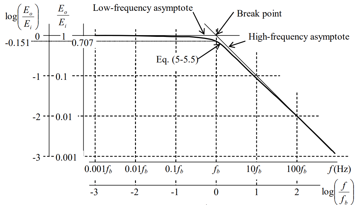
\[\frac{X(\omega)}{U}=\frac{b \tau_{1}}{\sqrt{1+\left(\omega \tau_{1}\right)^{2}}}=\frac{E_{o}(\omega)}{E_{i}}=\frac{1}{\sqrt{1+\left(\omega \tau_{1}\right)^{2}}}=\frac{1}{\sqrt{1+\left(\omega / \omega_{b}\right)^{2}}}\label{eqn:5.5.5} \]

and the standard FRF phase Equation 4.5.8 is adapted as \(\phi(\omega)=\tan ^{-1}\left(-\omega \tau_{1}\right)=\tan ^{-1}\left(-\omega / \omega_{b}\right)\) in which the break frequency is \(\omega_{b}=1 / \tau_{1}=1 / R C=2 \pi f_{b}\). Figure \(\PageIndex{6}\) (adapted from Figure 4.3.3) is the log-log graph of magnitude ratio versus frequency, which clearly shows the low-pass character of the frequency response.

Figure \(\PageIndex{6}\): Log-log magnitude ratio of 1^st order \(RC\) low-pass filter

The governing ODE of the mechanical series damper-spring low-pass filter in Figure 3.7.4 is Equation 3.7.5, \(\tau_{1} \dot{x}_{o}+x_{o}=x_{i}(t)\) (see also homework Problem 4.3), which has exactly the same form as Equation \(\ref{eqn:5.5}\). Accordingly, the electrical low-pass filter is an exact electrical analog of the mechanical low-pass filter, input voltage \(e_{i}(t)\) being directly analogous to input translation \(x_{i}(t)\), output voltage \(e_{o}(t)\) to output translation \(x_{o}(t)\), and electrical time constant \(\tau_{1}=R C\) to mechanical time constant \(\tau_{1}=c / k\).

Figure \(\PageIndex{7}\): Ideal inductor

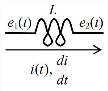
The passive electrical component drawn in Figure \(\PageIndex{7}\) represents an ideal linear inductor, with inductance \(L\) henry (H) in SI units. A time-varying current \(i(t)\) is shown flowing through the inductor. The graphical symbol denoting the inductor depicts a coil of conducting wire. If the current is changing with time in such a coil, then a voltage difference appears across the coil, a voltage difference that opposes the current change (Halliday and Resnick, 1960, Sections 36-1 and 36-3). This voltage difference is called a self-induced emf (electromotive force); it is a manifestation of the interaction between electricity and magnetism that is described by Maxwell’s equations of electromagnetism (after Scottish physicist James Clerk Maxwell, 1831-1879). The self-induced emf is proportional to the rate of change of current, with inductance \(L\) defined as the constant of proportionality:

\[e_{1}-e_{2}=L \frac{d i}{d t}\label{eqn:5.6} \]

You might find it difficult to perceive how Equation \(\ref{eqn:5.6}\) represents physically a voltage difference that opposes current change \(d i / d t\). If so, then the following example should illustrate this characteristic more understandably.

Example \(\PageIndex{4}\) - 1^st order \(LR\) circuit

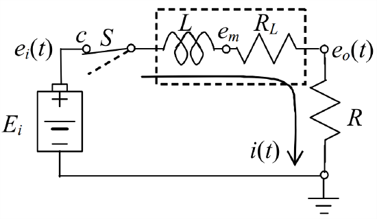
Real inductors are not used in instrumentation circuits nearly as often as resistors and capacitors. Moreover, there is no such thing as the ideal inductor instrumentation component of Figure \(\PageIndex{7}\). Because an inductor component consists primarily of coiled wire, and because a considerable length of very fine wire accumulates resistance, a real inductor usually has non-negligible resistance as well as inductance. A common, simple, approximate circuit model for such a real inductor is a series combination of an ideal inductor and a resistor, \(L\) and \(R_L\) in the circuit of Figure \(\PageIndex{8}\). In this circuit, \(e_{i}(t)\) is the input voltage (after switch \(S\) is closed to position \(c\)), and \(e_{o}(t)\) is the output voltage. \(R\) is a resistor placed between the inductor and ground to permit sensing (by an oscilloscope, for example) of \(e_{o}(t)\), which is directly related to the current by \(e_{o}(t)=R i(t)\).

Figure \(\PageIndex{8}\): \(LR\) circuit

Solution

Next, we derive an ODE governing the dynamic behavior of the \(LR\) circuit in Figure \(\PageIndex{8}\). Observe that the derivative of current, \(d i / d t\), appears in Equation \(\ref{eqn:5.6}\), unlike Equation \(\ref{eqn:5.1}\) for a resistor and Equation \(\ref{eqn:5.3}\) for capacitor, in which equations current \(i(t)\) appears directly. Because of this, it is usually not convenient to apply Kirchhoff’s current law for a circuit containing an inductor. It is usually better for such a circuit to apply Kirchhoff’s voltage law (abbreviated “KVL”): the sum of all voltage rises around a circuit loop is zero. If we proceed around the circuit loop in the direction of defined positive current flow, then the “voltage rise” across any component (including the input voltage generator and every passive component) is defined to be the upstream voltage minus the downstream voltage. To write KVL for this \(LR\) circuit, we start at the input voltage generator and proceed clockwise:

\[\left(e_{i}-0\right)+\left(e_{m}-e_{i}\right)+\left(e_{o}-e_{m}\right)+\left(0-e_{o}\right)=0\label{eqn:5.7} \]

Kirchhoff’s voltage law is a fundamental law of circuits, but note that it also is just an algebraic identity. Next, we substitute Equation \(\ref{eqn:5.6}\) and Ohm’s law into Equation \(\ref{eqn:5.7}\):

\[\left(e_{i}-0\right)+\left(-L \frac{d i}{d t}\right)+\left(-R_{L} i\right)+(-R i)=0 \Rightarrow L \frac{d i}{d t}+\left(R_{L}+R\right) i=e_{i}(t)\label{eqn:5.8} \]

Equation \(\ref{eqn:5.8}\) is a stable 1^st order LTI ODE solvable for arbitrary input voltage \(e_{i}(t)\). For example, suppose that all ICs = 0 and that the input voltage is a step, \(e_{i}(t)=E_{i} H(t)\), which is accomplished with use of a battery and a switch, as shown in Figure \(\PageIndex{8}\). Comparing Equation \(\ref{eqn:5.8}\) with standard stable 1^st order ODE Equation 3.4.8, we adapt the standard step-response solution Equation 3.4.9 with \(e_{i}(t) \equiv u(t)\) so that \(E_{i} \equiv U\), to write the electrical response quantities as

\[i(t)=\frac{E_{i}}{R_{L}+R}\left(1-e^{-t / \tau_{1}}\right), 0 \leq t \quad \text { in which } \quad \tau_{1}=\frac{L}{R_{L}+R}\label{eqn:5.9a} \]

\[\Rightarrow e_{o}(t)=R i(t)=\frac{R}{R_{L}+R} E_{i}\left(1-e^{-t / \tau_{1}}\right) \equiv E_{o}\left(1-e^{-t / \tau_{t}}\right), \quad E_{o} \equiv \frac{R}{R_{L}+R} E_{i}\label{eqn:5.9b} \]

Step response Equations \(\ref{eqn:5.9a}\) and \(\ref{eqn:5.9b}\) clearly show the effect of the inductance in opposing and delaying the rise of current flow. If the inductor were not present (i.e., if \(L\) = 0) in the circuit of Figure \(\PageIndex{8}\), then the circuit would be a simple voltage divider (Problem 5.1), and the full step-response output voltage would be achieved instantly, \(e_{o}(t)=E_{o} H(t)\), instead of rising gradually as in Equation \(\ref{eqn:5.9b}\).

The response of this circuit illustrates the physical effect of the inductor’s self-induced emf, Equation \(\ref{eqn:5.6}\). In this circuit, the inductor’s upstream voltage is constrained to be the input, \(e_{i}(t)\), so the self-induced emf must act in \(e_{m}(t)\), the voltage at the inductor’s downstream terminal. It is helpful to derive from Equations \(\ref{eqn:5.7}\), \(\ref{eqn:5.8}\), \(\ref{eqn:5.9a}\), and \(\ref{eqn:5.9b}\) the equation for that voltage, \(e_{m}(t)=e_{o}(t)+R_{L} i(t)=E_{i}\left(1-e^{-t / \tau_{T}}\right)\), and the equation for the rate of change of current, \(d i / d t=\left(E_{i} / L\right) e^{-t / \tau_{1}}\). At time \(t\) = \(0^+\) (just after switch \(S\) is closed to position \(c\)), we have \(d i / d t(0+)=E_{i} / L>0\) but \(e_{m}(0+)=0\) and \(i(0+)=0\). Thus, at this instant, the inductor holds its downstream voltage at zero and prevents the current from rising instantaneously as a step function, which it would do if the inductor were not present. After time \(t=0+\), the current gradually rises, but at a declining rate, and the current increase is still opposed by the inductor downstream voltage, which also rises at the same declining rate.

From Equation \(\ref{eqn:5.6}\), we have the unit equivalence \(\mathrm{V}=\mathrm{H} \times \frac{\mathrm{A}}{\mathrm{s}} \Rightarrow \mathrm{H}=\frac{\mathrm{V}-\mathrm{s} }{\mathrm{A}}\); this relation for the henry is useful for clarifying units in calculations, as shown in the following example. A particular “voice coil” is to be used in an electromagnetic force actuator; this is the type of wire coil found in the speakers of consumer sound systems. We wish to identify experimentally for this coil the parameters \(L\) and \(R_L\) (based upon the series model of Electricity Example 5.2.4) by measuring the step response of the circuit of Figure \(\PageIndex{8}\). For this particular circuit, the sensing resistor has \(R\) = 17.5 \(\Omega\), and the battery voltage is 9.00 V. We close switch \(S\), then record the subsequent time-history graphical response onto the screen of a digital oscilloscope, which stores the data for analysis. The response graph (below) has the appearance of Figure 3.4.2, and we measure from it the time

Figure \(\PageIndex{9}\)

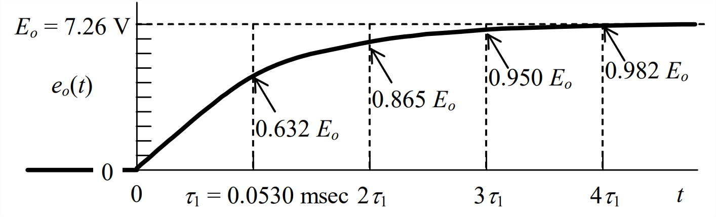
constant \(\tau_{1}=0.0530\) ms and the final value of output voltage Eo = 7.26 V. From the equations for \(\tau_{1}\) in Equation \(\ref{eqn:5.9a}\) and in Equation \(\ref{eqn:5.9b}\), we derive the following equations for the required parameters \(L\) and \(R_L\), and then the subsequent calculated values:

\[\begin{aligned}
L &=\left(R_{L}+R\right) \tau_{1}=\left(\frac{R}{E_{o}} E_{i}\right) \tau_{1} \\
&=\frac{E_{i}}{E_{o}} R \tau_{1}=\left(\frac{9.00 \mathrm{V}}{7.26 \mathrm{V}}\right)\left(17.5 \frac{\mathrm{V}}{\mathrm{A}}\right)\left(0.0530 \times 10^{-3} \mathrm{sec}\right)=1.15 \times 10^{-3} \frac{\mathrm{V}-\mathrm{sec}}{\mathrm{A}} \equiv 1.15 \mathrm{mH}
\end{aligned} \nonumber \]

\[R_{L}=\frac{R}{E_{o}} E_{i}-R=R\left(\frac{E_{i}}{E_{o}}-1\right)=(17.5 \Omega)\left(\frac{9.00 \mathrm{V}}{7.26 \mathrm{V}}-1\right)=4.19 \Omega \nonumber \]