Consider a mass-damper system with a suddenly applied cosine forcing function beginning at \(t\) = 0, and let the mass have a known initial velocity. The complete problem for velocity \(v(t)\) is described by the 1st order, LTI ODE \(m \dot{v}+c v=F \cos \omega t\), \(t\) > 0, and the IC \(v(0)=v_{0}\). Use the general solution Equation 6.2.4 to write an algebraic equation for the complete solution \(v(t)\) of this problem. It will be necessary to evaluate the convolution integral. You may use integration by parts and/or published tables of integrals, which are highly recommended. Symbolic software (Mathematica, MATLAB, etc.) is also a potential source of assistance with difficult integrals. \[\text {Answer: } v(t)=\left[v_{0}-\frac{F}{c} \frac{1}{1+\left(\omega \tau_{1}\right)^{2}}\right] e^{-t / \tau_{1}}+\frac{F}{c} \frac{1}{1+\left(\omega \tau_{1}\right)^{2}}\left(\cos \omega t+\omega \tau_{1} \sin \omega t\right), t \geq 0 \nonumber \]
Consider the standard 1st order LTI ODE (of a stable physical system) for dependent variable \(x(t): \quad \dot{x}+\left(1 / \tau_{1}\right) x=b u(t)\), with IC \(x(0)\) = 0. Let the input function be the following flat pulse of duration \(t_d\): \[u(t)=\left\{\begin{array}{ll}
0, & t<0 \\
U, & 0<t<t_{d}, \text { in which amplitude } U \text { is constant } \\
0, & t_{d}<t
\end{array}\right. \nonumber \]
Use solutions Equations 6.3.2 and 6.3.3 to write two algebraic equations for the complete response \(x(t)\) of this problem. One equation should apply for the time during which the pulse is active (including initial and final times), \(0 \leq t \leq t_{d}\), and the other equation should apply for the time after the pulse ceases, \(t_{d} \leq t\). It will be necessary to evaluate the convolution integral. \[\text {Answer: } x(t)=\left\{\begin{array}{l}
b U \tau_{1}\left(1-e^{-t / \tau_{1}}\right), \quad 0 \leq t \leq t_{d} \\
b U \tau_{1}\left(e^{-\left(t-t_{d}\right) / \tau_{1}}-e^{-t / \tau_{1}}\right), \quad t_{d} \leq t
\end{array}\right. \nonumber \] Note that the result for \(t_{d} \leq t\) can be written also as \[x(t)=b U \tau_{1}\left(1-e^{-t_{d} / \tau_{1}}\right) e^{-\left(t-t_{d}\right) / \tau_{1}}, \quad t_{d} \leq t \nonumber \]
Suppose that \(t_{d}=\tau_{1}\). Sketch by hand (not by computer) a reasonably accurate timehistory plot of the nondimensionalized output \(\frac{x(t)}{b U \tau_{1}}\) versus time over the time interval \(0 \leq t \leq 5 \tau_{1}\).
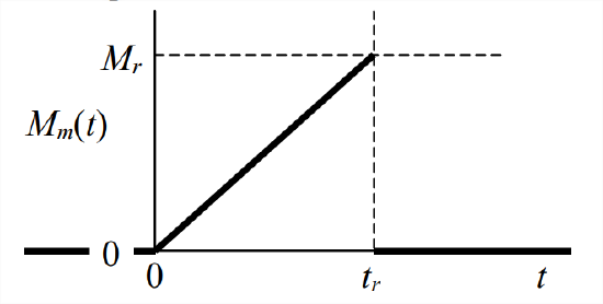
Consider the equation of motion for spin velocity \(p(t)\) of a reaction wheel (from Example 6.3 in Section 6.3): \(\dot{p}+\left(c_{\theta} / J\right) p=(1 / J) M_{m}(t)\), with IC \(p(0)=0\). Let the applied motor torque be the following sawtooth pulse: \[M_{m}(t)=\left\{\begin{array}{cc}
0, & t<0 \\
\frac{M_{r}}{t_{r}} t,& 0 \leq t<t_{r} \\
0, & t_{r}<t
\end{array}\right. \nonumber \]
Figure \(\PageIndex{1}\)
Use solutions Equations 6.3.2 and 6.3.3 to write two algebraic equations for the complete solution \(p(t)\) of this problem. One equation should apply for the time during which the pulse is active (including initial and final times), \(0 \leq t \leq t_{r}\), and the other equation should apply for the time after the pulse ceases, \(t_{r} \leq t\). You may and should use without re-derivation the appropriate results from Example 6.3 in Section 6.3, in which the applied moment is a permanently increasing ramp.
Use MATLABdemo61.m in Section 6.5 as a template (which must be revised and supplemented with labels, grids, etc.) to calculate approximately and graph the velocity response of the same mass-damper system with the same IC, but now specifying smaller (than in Section 6.5) calculation time steps: \(\Delta t\) = 0.5 s and \(\Delta t\) = 0.25 s. You should find that the calculated dynamic response becomes progressively more accurate as you reduce \(\Delta t\).
Derive a more accurate recurrence formula than Equation 6.5.5 by approximating \(u(\tau)\) as varying linearly with time over each time step. In other words, use in Equation 6.5.1 the linear approximation \[u(\tau) \approx u_{n-1}+\frac{\tau-t_{n-1}}{\Delta t}\left(u_{n}-u_{n-1}\right) \text { for } t_{n-1} \leq \tau \leq t_{n} \nonumber \] instead of the simpler approximation Equation 6.5.2. By completing the integration, show (in all detail, as if the answer were not given) that the refined version of Equation 6.5.5 is \[x_{n}=\phi x_{n-1}+\gamma u_{n-1}+\beta\left(u_{n}-u_{n-1}\right) \nonumber \] in which \(\phi\) and \(\gamma\) are the constants defined in Equation 6.5.5, and \(\beta \equiv \frac{\gamma}{a \Delta t}-\frac{b}{a}\).
Revise M-file MATLABdemo61.m of Section 6.5 to implement the refined recurrence formula of part 6.5.1. Using exactly the same numerical data as in the original program, run the revised program and plot the approximate time history \(v(t)\). The approximate time history calculated by the refined recurrence formula should be substantially more accurate than that calculated by Equation 6.5.5.
Consider the standard 1st order LTI-ODE of a stable system, Equation 3.4.8, for dependent variable \(x(t): \quad \dot{x}+\left(1 / \tau_{1}\right) x=b u(t)\). Let the initial condition be zero, \(x(0)=0\), and let the input function be a declining ramp, \(u(t)=c\left(t_{z}-t\right)\), in which \(c\), a dimensional constant, is the downward slope of the ramp, and \(t_z\) is the time at which the input passes through zero.
Evaluate in all detail the convolution integral in Equation 6.2.4 to show that the exact response solution is \(x(t)=b c \tau_{1}\left[\left(t_{z}+\tau_{1}\right)\left(1-e^{-t / \tau_{1}}\right)-t\right]=b c \tau_{1}\left[t_{z}+\tau_{1}-t-\left(t_{z}+\tau_{1}\right) e^{-t / \tau_{1}}\right]\).
Let the numerical parameters be \(\tau_1\) = 2.5 s, \(t_z\) = 10 s, \(b\) = 3.5, and \(c\) = 1 (\(b\) and \(c\) in consistent units). Write a MATLAB program, or adapt the code in Section 6.5 that executes the recurrence formula, to calculate and plot an approximate numerical solution for \(x(t)\) over the time interval \(0 \leq t \leq 10\) s. Adjust the time-step size \(\Delta\) and the number of time steps over the 10-s interval in your code until the graph of your approximate solution appears very similar to that of the corresponding exact solution from part 6.6.1. Submit your MATLAB code and your final graph of response.