8.4: Dirac Delta Function

Consider a limit process with the flat impulse of Fig. 8.3.1, in which process we progressively shorten the pulse duration while maintaining constant the impulse magnitude (the shaded area), thereby progressively increasing the input magnitude, \(I_{U} / t_{d}\). If we carry the process to the limit as \(t_{d} \rightarrow 0\) while maintaining \(I_{U}\) constant, then magnitude \(I_{U} / t_{d} \rightarrow \infty\). The limit process is illustrated on Figure \(\PageIndex{1}\). The function that results is called an ideal impulse with magnitude \(I_{U}\), and it is denoted as \(u(t)=I_{U} \times \delta(t)\), in which \(\delta(t)\) is called the Dirac delta function (after English mathematical physicist Paul Dirac, 1902-1984) or the unit-impulse function. The ideal impulse function \(I_{U} \delta(t)\) is usually depicted graphically by a thick picket at \(t\) = 0, as on Figure \(\PageIndex{1}\). With \(I_{U}=1\) in Equation 8.3.1, a formal mathematical definition of the unit-impulse function is

\[\delta(t)=\lim _{t_{d} \rightarrow 0} \frac{1}{t_{d}}\left[H(t)-H\left(t-t_{d}\right)\right]\label{eqn:8.8} \]

Observe from Equation \(\ref{eqn:8.8}\) that the dimension of \(\delta(t)\) is time^-1, since the unit-step is dimensionless, so the typical unit of \(\delta(t)\) is s^-1.

Figure \(\PageIndex{1}\): Ideal impulse

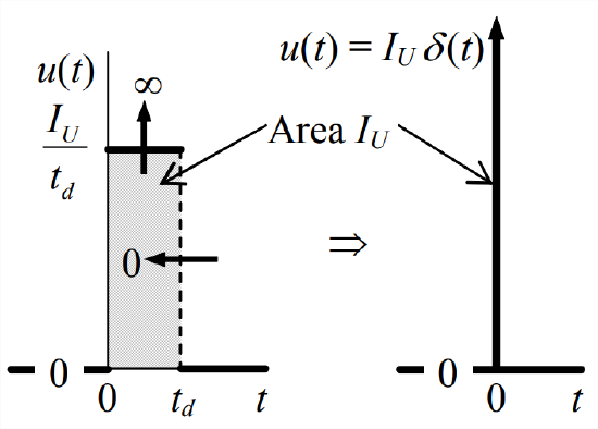
By definition, the area under \(u(t)=I_{U} \delta(t)\) equals \(I_{U}\), so the area under \(\delta(t)\) equals 1 (hence the name unit-impulse function). This unit area under an infinitely short impulse suggests an important effect of the Dirac delta function in integrands. In order to describe this effect, we define a more general unit-impulse function, \(\delta\left(t-t_{\delta}\right)\), which peaks infinitely at some arbitrary time \(t_{\delta}\) that is not necessarily zero; otherwise, the nature of \(\delta\left(t-t_{\delta}\right)\) is identical to that of \(\delta(t)\) [in fact, \(\delta(t)=\delta\left(t-t_{\delta}\right)\) for \(t_{\delta}\) = 0]. Now suppose that we have some realistic physical function \(f(t)\) that is defined over the time interval \(t_{1} \rightarrow t_{2}\), and suppose that time \(t_{\delta}\) is within this interval, as in the figure below. Then the useful integration effect of \(\delta\left(t-t_{\delta}\right)\) is:

\[\int_{t=t_{1}}^{t=t_{2}} f(t) \delta\left(t-t_{\delta}\right) d t=f\left(t_{\delta}\right) \label{eqn:8.9} \]

Figure \(\PageIndex{2}\)

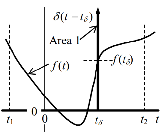
Equation \(\ref{eqn:8.9}\) states that, as a multiplier within the integrand, \(\delta\left(t-t_{\delta}\right)\) essentially “selects” the value of \(f(t)\) at \(t=t_{\delta}\). Result Equation \(\ref{eqn:8.9}\) is intuitively clear, and it can be proved more rigorously with the theory of so-called generalized functions (Lighthill, 1958).

If the upper limit of integration in Equation \(\ref{eqn:8.9}\) is an arbitrary time \(t>t_{\delta}\), then the result is a step function:

\[\int_{\tau=t_{1}}^{\tau=t>t_{\delta}} f(\tau) \delta\left(\tau-t_{\delta}\right) d \tau=f\left(t_{\delta}\right) H\left(t-t_{\delta}\right)\label{eqn:8.10} \]

Setting \(f(\tau)=1\) in Equation \(\ref{eqn:8.10}\) leads to a fundamental integral relationship between the unit-impulse function and the unit-step function:

\[\int_{\tau=t_{1}}^{\tau=t>t_{\delta}} \delta\left(\tau-t_{\delta}\right) d \tau=H\left(t-t_{\delta}\right)\label{eqn:8.11} \]

Figure \(\PageIndex{3}\)

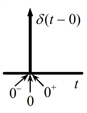
Next, we use Equation \(\ref{eqn:8.9}\) to derive the Laplace transform of delta function \(\delta(t)= \delta(t-0)\). According to the definition of Equation 2.2.5, this transform would be written as \(L[\delta(t)]=\int_{t=0}^{t=\infty} e^{-s t} \delta(t-0) d t\); however, there is a problem with this particular definition: at \(t\) = 0, which is the lower limit of the integrand (and the initial-value instant for most ODEs that we solve using Laplace transforms), the function \(\delta(t-0)\) is nominally infinite, so the meaning of the integral is uncertain. We choose to remove the uncertainty by specifying that \(\delta(t-0)\) must lie within the limits of the integration. In order to indicate this clearly in notation, we now define three different reference instants, as depicted on the drawing at right:

1. \(t=0^{-}\), the instant just before activity of the ideal impulse function, at and before which \(\delta(t-0)=0\);
2. \(t = 0\), the instant when \(\delta(t-0)\) acts and is nominally infinite; and
3. \(t=0^{+}\), the instant just after activity of the ideal impulse function, at and after which \(\delta(t-0)=0\).

Accordingly, we re-define the Laplace transform, more generally than in Equation 2.2.5, as

\[L[f(t)]=\int_{t=0^{-}}^{t=\infty} e^{-s t} f(t) d t\label{eqn:8.12} \]

The distinction between \(t=0\) and \(t=0^-\) in the lower limits of Equations 2.2.5 and \(\ref{eqn:8.12}\), respectively, is meaningless for all problems considered in this book except those in which \(f(t)\) involves an ideal impulse function. Application of Equations \(\ref{eqn:8.9}\) and \(\ref{eqn:8.12}\) now leads to the Laplace transform of the basic ideal impulse function:

\[L[\delta(t)]=\int_{t=0^{-}}^{t=\infty} e^{-s t} \delta(t-0) d t=e^{-s \times 0}=1\label{eqn:8.13} \]