9.7: Ideal Impulse Response of Underdamped Second Order Systems

Last updated
Save as PDF

Page ID: 8343

\( \newcommand{\vecs}[1]{\overset { \scriptstyle \rightharpoonup} {\mathbf{#1}} } \) \( \newcommand{\vecd}[1]{\overset{-\!-\!\rightharpoonup}{\vphantom{a}\smash {#1}}} \)\(\newcommand{\id}{\mathrm{id}}\) \( \newcommand{\Span}{\mathrm{span}}\) \( \newcommand{\kernel}{\mathrm{null}\,}\) \( \newcommand{\range}{\mathrm{range}\,}\) \( \newcommand{\RealPart}{\mathrm{Re}}\) \( \newcommand{\ImaginaryPart}{\mathrm{Im}}\) \( \newcommand{\Argument}{\mathrm{Arg}}\) \( \newcommand{\norm}[1]{\| #1 \|}\) \( \newcommand{\inner}[2]{\langle #1, #2 \rangle}\) \( \newcommand{\Span}{\mathrm{span}}\) \(\newcommand{\id}{\mathrm{id}}\) \( \newcommand{\Span}{\mathrm{span}}\) \( \newcommand{\kernel}{\mathrm{null}\,}\) \( \newcommand{\range}{\mathrm{range}\,}\) \( \newcommand{\RealPart}{\mathrm{Re}}\) \( \newcommand{\ImaginaryPart}{\mathrm{Im}}\) \( \newcommand{\Argument}{\mathrm{Arg}}\) \( \newcommand{\norm}[1]{\| #1 \|}\) \( \newcommand{\inner}[2]{\langle #1, #2 \rangle}\) \( \newcommand{\Span}{\mathrm{span}}\)\(\newcommand{\AA}{\unicode[.8,0]{x212B}}\)

For impulse response, we set the ICs to zero, and we define the input to be an ideal impulse at time \(t = 0\), with impulse magnitude \(I_{U}\): \(u(t)=I_{U} \delta(t)\). The more appropriate form of the general solution to use is Equation 9.3.9, which becomes

\[x(t)=\frac{\omega_{n}^{2}}{\omega_{d}} \int_{\tau=0}^{\tau=t} e^{-\zeta \omega_{n}(t-\tau)} \sin \omega_{d}(t-\tau) \times u(\tau) d \tau=\frac{\omega_{n}^{2}}{\omega_{d}} \int_{\tau=0}^{\tau=t} e^{-\zeta \omega_{n}(t-\tau)} \sin \omega_{d}(t-\tau) \times I_{U} \delta(\tau) d \tau \nonumber \]

Using the integration property of \(\delta(\tau)\), Equation 8.4.4, we find the relatively simple result:

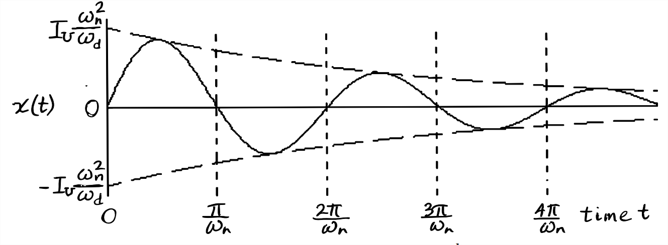
\[x(t)=I_{U} \frac{\omega_{n}^{2}}{\omega_{d}} e^{-\zeta \omega_{n} t} \sin \omega_{d} t, \text { for } 0<t \text { and } 0 \leq \zeta<1\label{eqn:9.30} \]

Ideal impulse response Equation \(\ref{eqn:9.30}\) for small damping ratio \(\zeta= 0.11\) is plotted over a few cycles of response on Figure \(\PageIndex{1}\). Observe that this ideal response violates the specified initial condition \(\dot{x}(0)=0\); thus, the solution is defective in this respect, as is discussed in Section 8.7. Figure \(\PageIndex{1}\) shows the exponential envelope; note, in particular, the values at \(t = 0\) of the exponential envelope, \(\pm I_{U} \omega_{n}^{2} / \omega_{d}\). This magnitude is easily measurable from a graph, after we have sketched in the exponential envelope, if necessary, and it is essential in the process of estimating mechanical system parameters from an experimental response to a short force pulse (Section 9.9).

Figure \(\PageIndex{1}\): Ideal impulse response of a damped 2^nd order system, \(\zeta = 0.11\)

From Equation Equation \(\ref{eqn:9.30}\), we find the unit-impulse-response function (IRF, as defined in Section 8.7) for underdamped 2^nd order systems:

\[\left.h(t) \equiv x(t)\right|_{I_{U}=1}=\frac{\omega_{n}^{2}}{\omega_{d}} e^{-\zeta \omega_{n} t} \sin \omega_{d} t, \text { for } 0<t \text { and } 0 \leq \zeta<1\label{eqn:9.31} \]

Further, from Equation 8.7.2, we find the Duhamel integral giving general response to input \(u(t)\), with zero ICs, for underdamped 2^nd order systems:

\[\left.x(t)\right|_{I C s=0}=\int_{\tau=0}^{\tau=t} u(\tau) h(t-\tau) d \tau=\frac{\omega_{n}^{2}}{\omega_{d}} \int_{\tau=0}^{\tau=t} u(\tau) e^{-\zeta \omega_{n}(t-\tau)} \sin \omega_{d}(t-\tau) d \tau\label{eqn:9.32} \]

Duhamel integral Equation \(\ref{eqn:9.32}\) is identical to convolution-integral response solution Equation 9.3.9 with zero ICs.

Finally, it is worthy of mention that convolution sum Equation 8.11.4 for approximate numerical forced response applies just as well to damped 2^nd order systems as to 1^st order and undamped 2^nd order systems. Therefore, to calculate approximate forced response of an underdamped 2^nd order system, we would apply exactly the same procedure described in Convolution-sum Example 2 of Section 8.11, but instead of calculating in Equation 8.11.4 the IRF \(h(t)=\omega_{n} \sin \omega_{n} t\) for an undamped system, we would calculate Equation \(\ref{eqn:9.31}\).