10.1: Frequency Response of Undamped Second Order Systems and Resonance

As discussed in Section 7.1, a truly undamped 2^nd order passive system is physically unrealistic. Nevertheless, it is useful to derive the frequency response for this ideal type of system because the results reveal important characteristics of the resonating behavior of general underdamped 2^nd order systems. Moreover, the frequency response of an undamped 2^nd order system is, for many practical purposes, a simple yet satisfactory engineering approximation to the frequency response of the corresponding lightly damped 2^nd order system.

Consider the standard ODE for idealized undamped 2^nd order systems:

\[\ddot{x}+\omega_{n}^{2} x=\omega_{n}^{2} u(t)\label{eqn:10.1} \]

To derive frequency response, we let \(u(t)=U \cos \omega t\) and seek the steady-state sinusoidal response in the form \(x(t)=X_{S}(\omega) \cos \omega t\), in which \(X_{S}(\omega)\) is the unknown quantity. We find an equation for \(X_{S}(\omega)\) by substituting into Equation \(\ref{eqn:10.1}\):

\[\left(-\omega^{2}+\omega_{n}^{2}\right) X_{S}(\omega) \cos \omega t=\omega_{n}^{2} U \cos \omega t \nonumber \]

\[\Rightarrow \frac{X_{S}(\omega)}{U}=\frac{\omega_{n}^{2}}{\omega_{n}^{2}-\omega^{2}}=\frac{1}{1-\left(\omega / \omega_{n}\right)^{2}}\label{eqn:10.2} \]

Note from Equation \(\ref{eqn:10.2}\) that \(X_{S}(\omega)\) is a signed quantity; it can be positive or negative depending upon the value of frequency ratio \(\omega / \omega_{n}\) relative to 1. But our conventional notation for a frequency response function is \(F R F(\omega)=\frac{X(\omega)}{U} e^{j \phi(\omega)}\), Equation 7.7.18, in which magnitude \(X(\omega) \geq 0\). Therefore, we infer from Equation \(\ref{eqn:10.2}\) the following magnitude-ratio and phase functions in the conventional notation:

\[\frac{X(\omega)}{U}=\left|\frac{1}{1-\left(\omega / \omega_{n}\right)^{2}}\right|, \phi(\omega)=\left\{\begin{array}{r}
0^{\circ} \text { for } 0 \leq \omega / \omega_{n}<1 \\
-180^{\circ} \text { for } 1<\omega / \omega_{n}
\end{array}\right.\label{eqn:10.3} \]

Equations \(\ref{eqn:10.3}\) give the frequency response function (FRF) of an undamped 2^nd order system. The magnitude ratio \(X(\omega) / U\) and phase \(\phi(\omega)\) are plotted on Figure \(\PageIndex{1}\) as functions of excitation frequency ratio \(\omega / \omega_{n}\).

The most important feature of FRF Equations \(\ref{eqn:10.3}\) is the infinite magnitude of steady-state response when excitation frequency \(\omega\) exactly equals natural frequency \(\omega_n\). This is the extreme version of the phenomenon called resonance. In reality, any damping, no matter how small, reduces the infinite resonance magnitude of Fig. 10-1 to some finite value, as is demonstrated in the next section; but that finite value will still generally be much greater than the static or pseudo-static response, which is \(X(\omega \approx 0)=U\). Figure \(\PageIndex{1}\) shows also that the response magnitude is greatly amplified relative to static response even if the excitation frequency is close (but not equal) to the natural frequency; note, for example, that the dynamic amplification exceeds five (5) whenever excitation frequency \(\omega\) is within about \(\pm\)10% of natural frequency \(\omega_n\). This high sensitivity to excitation near the natural frequency is a very important characteristic of lightly damped 2^nd order systems. There is additional discussion of resonance in the next section.

Figure \(\PageIndex{1}\): Frequency response function of an undamped 2^nd order system

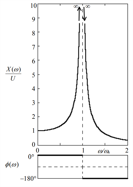
FRF Equations \(\ref{eqn:10.3}\) contains not only the magnitude but also the phase \(\phi\): for \(\omega<\omega_{n}\), the phase is 0°, so the response is exactly in phase with the excitation; however, for \(\omega>\omega_{n}\), the phase is −180°, so the response is exactly out of phase with the excitation.