10.2: Frequency Response of Damped Second Order Systems

From Section 9.2, the standard form of the 2 ^nd order ODE is:

\[\ddot{x}+2 \zeta \omega_{n} \dot{x}+\omega_{n}^{2} x=\omega_{n}^{2} u(t) \label{eqn:10.4} \]

To derive frequency response, we take the Laplace transform of Equation \(\ref{eqn:10.4}\), with zero ICs:

\[\left.\left(s^{2}+2 \zeta \omega_{n} s+\omega_{n}^{2}\right) L[x(t)]\right|_{I C s=0}=\omega_{n}^{2} L[u(t)]\label{eqn:10.5} \]

Definition Equation 4.6.3 for the transfer function gives

\[T F(s)=\frac{\left.L[x(t)]\right|_{I C s=0}}{L[u(t)]}=\frac{\omega_{n}^{2}}{s^{2}+2 \zeta \omega_{n} s+\omega_{n}^{2}}\label{eqn:10.6} \]

Then the fundamental relationship Equation 4.7.18 between the transfer function and the complex frequency response function gives

\[F R F(\omega)=T F(j \omega)=\frac{\omega_{n}^{2}}{-\omega^{2}+j 2 \zeta \omega_{n} \omega+\omega_{n}^{2}}=\frac{1}{\left(1-\omega^{2} / \omega_{n}^{2}\right)+j 2 \zeta \omega / \omega_{n}}\label{eqn:10.7} \]

To simplify notation, we define the dimensionless excitation frequency ratio, the excitation frequency relative to the system undamped natural frequency:

\[\beta \equiv \frac{\omega}{\omega_{n}}\label{eqn:10.8} \]

With notation Equation \(\ref{eqn:10.8}\), the relationship Equation 4.7.18 between \(F R F(\omega)\) and the magnitude ratio \(X(\omega) / U\) and phase angle \(\phi(\omega)\) of the frequency response gives

\[F R F(\omega)=\frac{1}{\left(1-\beta^{2}\right)+j 2 \zeta \beta}=\frac{X(\omega)}{U} e^{j \phi(\omega)}\label{eqn:10.9} \]

After the standard manipulation of the complex fraction in Equation \(\ref{eqn:10.9}\), we find the following equations for magnitude ratio and phase angle [homework Problem 2.6.1]:

\[\frac{X(\omega)}{U}=\frac{1}{\sqrt{\left(1-\beta^{2}\right)^{2}+(2 \zeta \beta)^{2}}}, \quad \phi(\omega)=\tan ^{-1}\left(\frac{-2 \zeta \beta}{1-\beta^{2}}\right), \quad \beta \equiv \frac{\omega}{\omega_{n}}\label{eqn:10.10} \]

Note that results Equations \(\ref{eqn:10.10}\) are valid for any non-negative value of viscous damping ratio, \(\zeta \geq 0\); unlike most of the time-response equations derived in Chapter 9, Equations \(\ref{eqn:10.10}\) alone apply for underdamped, critically damped, and overdamped 2^nd order systems.

Results Equations \(\ref{eqn:10.10}\) are plotted on Figure \(\PageIndex{1}\) for viscous damping ratios varying from 0 to 1. The graphs of Figure \(\PageIndex{1}\) were produced with use of MATLAB (Version 6 or later). First, an M-file was programmed to calculate and graph FRFs using the method described in the statement of homework Problem 4.3 [starting with complex FRF Equation \(\ref{eqn:10.9}\)), not the real equations Equations \(\ref{eqn:10.10}\)]:

%frf2orddamped.m

%Fig. 10-2 Frequency response, damped 2nd order

%Magnitude ratio for zero damping, zeta=0

bt0a=logspace(-1,log10(0.998),100);

frf0a=(1)./(1-bt0a.^2);

loglog(bt0a,frf0a,'k'),hold on

bt0b=logspace(log10(1.002),1,100);

frf0b=(1)./(bt0b.^2-1);

loglog(bt0b,frf0b,'k')

%Magnitude ratio for several cases of zeta > 0

bt1=logspace(-1,1,400);

zt=[ 0.05 0.1 0.2 0.5 1/sqrt(2) 1];nzts=length(zt);

for i=1:nzts

frf=(1)./(1-bt1.^2+j*2*zt(i).*bt1);

magrat=abs(frf);

loglog(bt1,magrat,'k')

end

hold off

%Phase angle in degrees for zero damping, zeta=0

bt0a=[0.1 1];faz0a=zeros(1,2);

figure,semilogx(bt0a,faz0a,'k'),hold on

bt0b=[1 10];faz0b=-180*ones(1,2);

semilogx(bt0b,faz0b,'k')

%Phase angle in degrees for several cases of zeta > 0

for i=1:nzts

frf=(1)./(1-bt1.^2+j*2*zt(i).*bt1);

faz=angle(frf)*180/pi;

semilogx(bt1,faz,'k')

end

After the M-file was executed, the extensive figure editing features of MATLAB were used to set axis limits and to generate titles, labels, and curve annotations.

Even though Figure \(\PageIndex{1}\) was produced by computer-aided graphics, it is still important that you understand how to evaluate Equations \(\ref{eqn:10.10}\) with a hand calculator. These equations appear simple, but they can be tricky, particularly for the special case \(\zeta=0\). See homework Problem 2.6.2 for help with understanding how to evaluate Equations \(\ref{eqn:10.10}\) numerically.

There are several noteworthy characteristics of the frequency response of damped 2^nd order systems, from Equations \(\ref{eqn:10.10}\) and Figure \(\PageIndex{1}\):

• Resonance: maximum (peak) magnitude ratio The frequency at which the peak magnitude ratio occurs is called the resonance frequency, denoted \(\omega_{r}\), and this frequency is lower than natural frequency \(\omega_{n}\) if damping is positive, \(\zeta>0\). To find the maximum, we differentiate the magnitude ratio of Equations \(\ref{eqn:10.10}\), set the result to zero, and solve for the associated frequency (you can verify the result yourself, or see Meirovitch, 2001, pp. 115-116 for the details of calculus and algebra; also, there are instructive alternative approaches in Ogata, 1998, pp. 480-481 and in Clark, 1962, pp. 316-322):\[\frac{d}{d \beta}\left(\frac{X(\beta)}{U}\right)=0 \Rightarrow \beta_{r}=\sqrt{1-2 \zeta^{2}} \Rightarrow \omega_{r}=\omega_{n} \sqrt{1-2 \zeta^{2}}\label{eqn:10.11} \]Subscript \(r\) in Equation \(\ref{eqn:10.11}\) denotes a resonance quantity corresponding to the peak magnitude ratio \(X_{r} / U\). The excitation frequency must be real and greater than or equal to zero, so \(\omega_{r}=\omega_{n} \sqrt{1-2 \zeta^{2}}\) is valid only for \(0 \leq \zeta \leq 1 / \sqrt{2}=0.707\). If \(\zeta\) is positive but very small, then \(X_{r} / U\) occurs almost at the natural frequency, \(\omega_{r} \approx \omega_{n}\). As \(\zeta\) increases from very small positive values, \(\omega_{r}\) decreases until, for \(\zeta=1 / \sqrt{2}\), \(\omega_{r}=0\). However, dynamic amplification is insignificant for values of \(\zeta\) greater than about 0.5. Substituting Equation \(\ref{eqn:10.11}\) back into \(X(\omega) / U\) of Equations \(\ref{eqn:10.10}\) gives (after more algebra) the resonance value:\[\frac{X\left(\beta_{r}\right)}{U}=\frac{X_{r}}{U}=\frac{1}{2 \zeta \sqrt{1-\zeta^{2}}}\label{eqn:10.12} \]Note from Equation \(\ref{eqn:10.12}\) that for \(\zeta=1 / \sqrt{2}\) [the maximum permissible value for validity of Equation \(\ref{eqn:10.11}\)], we have \(X_{r} / U=1\) at \(\omega_{r}=0\). As indicated by the trend on Figure \(\PageIndex{1}\), for higher damping ratios, \(\zeta \geq 1 / \sqrt{2}\), the magnitude \(X(\omega) / U\) is maximum at \(\omega=0\), and decreases monotonically as \(\omega\) increases.

  

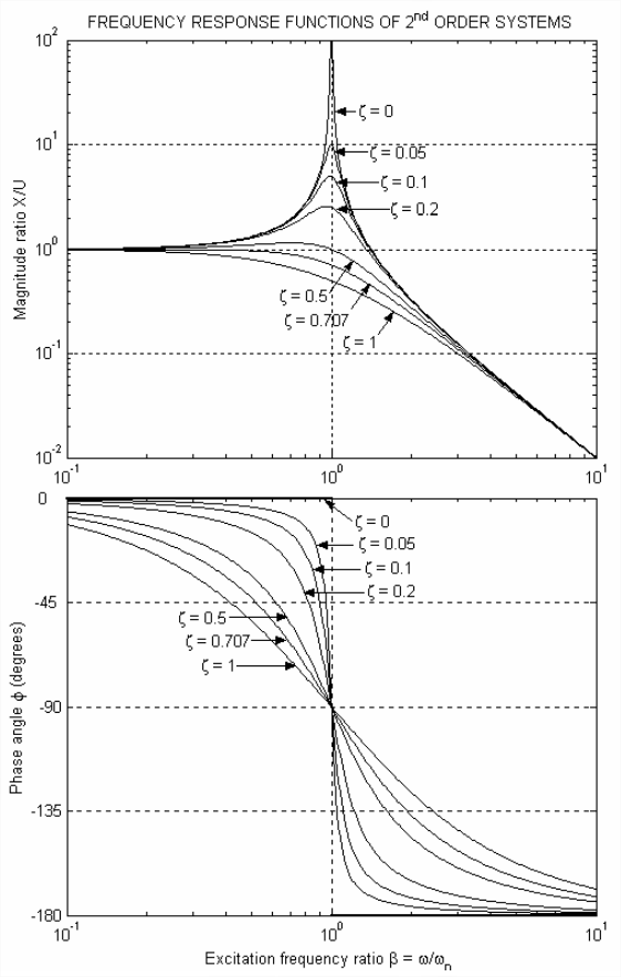
  Figure \(\PageIndex{1}\): Frequency response functions for standard 2^nd order systems with viscous damping ratios \(\zeta\) varying from 0 to 1

• Response at the natural frequency The frequency response at \(\omega=\omega_{n}\), \(\beta=1\), consists of phase angle \(\phi\left(\omega_{n}\right)=-90^{\circ}\) regardless of the value of viscous damping ratio \(\zeta\), and magnitude ratio \(X\left(\omega_{n}\right) / U=1 /(2 \zeta)\). Also, the peak magnitude response occurs essentially at \(\omega=\omega_{n}\) if damping is small, as discussed next.
• Small viscous damping, small-\(\zeta\) approximation If damping is so small that \(\sqrt{1-2 \zeta^{2}}\approx 1\), then we can use the following accurate approximations of the values associated with response at resonance, from Equations \(\ref{eqn:10.11}\) and \(\ref{eqn:10.12}\):\[\omega_{r}=\omega_{n} \sqrt{1-2 \zeta^{2}} \approx \omega_{n}\label{eqn:10.13} \]\[\frac{X_{r}}{U}=\frac{1}{2 \zeta \sqrt{1-\zeta^{2}}} \approx \frac{X\left(\omega_{n}\right)}{U}=\frac{1}{2 \zeta}\label{eqn:10.14} \]The upper limit of viscous damping ratio for which the small-\(\zeta\) approximation is practically useful is about \(\zeta=0.2\), which we can see on Figure \(\PageIndex{1}\). At this upper limit, the approximation is in error on the order of 4%, since \(\sqrt{1-2(0.2)^{2}}=0.959\). The small-\(\zeta\) resonance amplification factor Equation \(\ref{eqn:10.14}\) is sometimes called the quality factor, and it is denoted \(Q=1 /(2 \zeta)\). The “quality” reference is to tuning, especially of a receiving device such as a radio (Hammond, 1961, pp. 106-114). When you turn the analog tuning dial of an old radio, you are varying the value of capacitance in an \(LRC\) electrical tuning circuit in order to produce resonance with the electromagnetic carrier signal, which gives the strongest possible reception. Clearly, a high \(Q\) is desirable in the tuning circuit of a radio. On the other hand, high \(Q\) is often undesirable in mechanical systems, because it can lead to structural failure or other negative consequences. For example, if the system consisting of a car’s tire, suspension spring, and damping strut happens to resonate with the waves in a washboard dirt road, then the resulting vibration will produce poor ride quality and might even break car parts.

  Note on the Figure \(\PageIndex{1}\) graph of magnitude ratio that the \(\zeta=0\) curve bounds the curves for all \(\zeta>0\), and that it provides a good approximation for small \(\zeta\) at all frequencies except those close to \(\omega_{n}\); for small damping, therefore, the simple equation (10-3a) for magnitude ratio will, for some calculations, be sufficiently accurate.

• Phase angles of frequency response Figure \(\PageIndex{1}\) shows that the more lightly damped a system is, the closer its response is to being in phase with excitation below the natural frequency, and out of phase with excitation above the natural frequency. Furthermore, for excitation at the natural frequency, \(\omega=\omega_{n}\), response lags excitation by exactly 90°, regardless of the level of viscous damping; this so-called quadrature phase is an important characteristic often used to help determine natural frequencies in vibration testing of machines and structures.
• 2^nd order low-pass filter A moderately damped (\(0.5 \leq \zeta \leq 1\)) 2^nd order system can function as a low-pass filter, with natural frequency \(\omega_{n}\) being the break (corner) frequency. Compare the magnitude ratio curve for \(\zeta=1 / \sqrt{2}=0.707\) on Figure \(\PageIndex{1}\) with the magnitude ratio curve for a 1^st order low-pass filter, Figure 4.3.3. The most significant difference between the two curves is in their high-frequency asymptotes: the 2^nd order magnitude ratio rolls off at the rate of two decades for each decade increase of frequency (40 dB/decade rolloff), twice as steeply as the 1^st order magnitude ratio. Thus, the 2^nd order filter functions much more effectively than the 1^st order filter. However, an important practical deficiency (in some potential applications) of both types of low-pass filters is that they impose on the low-passed output large phase lags relative to the input.