10.6: Beating Response of Second Order Systems to Suddenly Applied Sinusoidal Excitation

Thus far in Chapter 10, we have considered only the pure frequency response of 2^nd order systems, i.e., the steady-state sinusoidal response to sinusoidal excitation. In frequency-response analysis based upon Equation 4.7.18, initial conditions are ignored, as is any non-steady-sinusoidal start-up portion of the excitation; in other words, both pure sinusoidal excitation and response are idealized to start at some indefinite time in the past. But any real excitation must start at some definite time, at which time any real dynamic system has some initial conditions. After the initiation of sinusoidal excitation, there will be a transitional interval of response between the initial conditions and, provided the system is stable, the achievement of steady-state sinusoidal response. Section 4.2 illustrates such a transitional interval for a stable 1^st order system, which does not exhibit natural oscillatory behavior. In this section, we consider a form of transitional response, beating, that is often observed in lightly damped vibrating systems, the simplest forms of which are underdamped 2^nd order systems.

The basic character of beating response to sinusoidal excitation is best illustrated theoretically by the idealized undamped 2^nd order system. Consider again the standard ODE for undamped 2^nd order systems, Equation 10.1.1. Suppose now that \(u(t)=0\) for \(t < 0\), and let us define the suddenly applied sinusoidal (SAS) excitation as \(u(t)=U \sin \omega t\) for \(t\geq 0\). (We use \(\sin \omega t\) here rather than the customary \(\cos \omega t\) because it is more natural, especially for mechanical systems, that the excitation begins continuously from zero at \(t\) = 0, rather than with a discontinuity.) Thus, the ODE Equation 10.1.1 becomes

\[\ddot{x}+\omega_{n}^{2} x=\omega_{n}^{2} u(t)=\omega_{n}^{2} U \sin \omega t, \text { for } t \geq 0\label{eqn:10.36} \]

For simplicity, we let the initial conditions be zero: \(\dot{x}(0)=0\) and \(x(0)=0\). The complete algebraic solution of ODE Equation \(\ref{eqn:10.36}\) with these rest ICs is found in homework Problem 1.12 by the method of undetermined coefficients:

\[x(t)=\frac{U}{1-\left(\omega / \omega_{n}\right)^{2}}\left[\sin \omega t-\left(\omega / \omega_{n}\right) \sin \omega_{n} t\right], \text { valid for } \omega \neq \omega_{n}, t \geq 0\label{eqn:10.37} \]

Equation \(\ref{eqn:10.37}\) is valid only if the excitation frequency is different than the natural frequency, \(\omega \neq \omega_{n}\); however, this is not a serious practical restriction, because it is almost impossible in reality to excite a system exactly at its natural frequency. [But see homework Problem 1.12.4 for the theoretical solution valid if \(\omega=\omega_{n}\).]

It is appropriate to write the response solution Equation \(\ref{eqn:10.37}\) in a slightly different algebraic form:

\[x(t)=\frac{U}{1-\left(\omega / \omega_{n}\right)^{2}}\left[\sin \omega t-\sin \omega_{n} t+\left(1-\omega / \omega_{n}\right) \sin \omega_{n} t\right]\label{eqn:10.38} \]

This form of \(x(t)\) allows us to invoke a useful trigonometric identity:

\[\sin \omega t-\sin \omega_{n} t=2 \cos \frac{1}{2}\left(\omega t+\omega_{n} t\right) \times \sin \frac{1}{2}\left(\omega t-\omega_{n} t\right)\label{eqn:10.39} \]

Now we can express the solution Equation \(\ref{eqn:10.38}\) in an equation that more clearly displays the characteristics of beating:

\[x(t)=\frac{U}{1-\left(\omega / \omega_{n}\right)^{2}}\left[2 \cos \frac{1}{2}\left(\omega+\omega_{n}\right) t \times \sin \frac{1}{2}\left(\omega-\omega_{n}\right) t+\left(1-\omega / \omega_{n}\right) \sin \omega_{n} t\right]\label{eqn:10.40} \]

For computation, with definitions of driving frequency ratio \(\beta \equiv \omega / \omega_{n}\) and natural period \(T_{n} \equiv 2 \pi / \omega_{n}\), we express Equation \(\ref{eqn:10.40}\) in the dimensionless form:

\[\frac{x(t)}{U}=\frac{1}{1-\beta^{2}}\left[2 \cos \left((\beta+1) \pi \frac{t}{T_{n}}\right) \times \sin \left((\beta-1) \pi \frac{t}{T_{n}}\right)+(1-\beta) \sin \left(2 \pi \frac{t}{T_{n}}\right)\right]\label{eqn:10.41} \]

Let us use numerical evaluation and graphical display to help us examine the parts of Equations \(\ref{eqn:10.40}\) and \(\ref{eqn:10.41}\); Figure \(\PageIndex{1}\) on the next page includes plots of both suddenly applied sinusoidal excitation and the associated response calculated from Equation \(\ref{eqn:10.41}\), with the excitation frequency set at 90% of the natural frequency, \(\omega=0.9 \omega_{n}\) or \(\beta=0.9\).

With use of Figure \(\PageIndex{1}\), we can identify the roles of the terms within square brackets of Equations \(\ref{eqn:10.40}\) and \(\ref{eqn:10.41}\) for any case in which the excitation frequency \(\omega\) is somewhat close to the system natural frequency \(\omega_{n}\). The dominant (in magnitude) term that closely resembles the excitation is \(2 \cos \frac{1}{2}\left(\omega+\omega_{n}\right) t\), a sinusoid whose frequency is the average of the excitation and natural frequencies. But this dominant term is multiplied by \(\sin \frac{1}{2}\left(\omega-\omega_{n}\right) t\), which is a slowly varying amplitude modulator whose frequency is half the difference between the excitation and natural frequencies. For the case of Figure \(\PageIndex{1}\) with \(\omega / \omega_{n}=0.9\), we have \(\left|\frac{1}{2}\left(\omega-\omega_{n}\right)\right|=0.05 \omega_{n}\). Therefore, the full period of the amplitude-modulating term is \(2 \pi / 0.05 \omega_{n}=20 T_{n}\); from Figure \(\PageIndex{1}\), this period is the total interval between time \(t = 0\) s and the second subsequent minimum of the amplitude-modulating envelope. Furthermore, the beating terms are minimal in amplitude at every half-period of the amplitude-modulating term, in this case \(0,10 T_{n}, 20 T_{n}, \ldots\), and the beating terms are maximal in amplitude at instants between the half-period instants, in this case \(5 T_{n}, 15 T_{n}, 25 T_{n}, \ldots\)

Figure \(\PageIndex{1}\): Upper graph: suddenly applied (at \(t = 0\)) sinusoidal (SAS) excitation with frequency \(\omega=0.9 \omega_{n}\); lower graph: response from zero initial conditions of a standard undamped 2^nd order system having natural frequency \(\omega_{n}\).

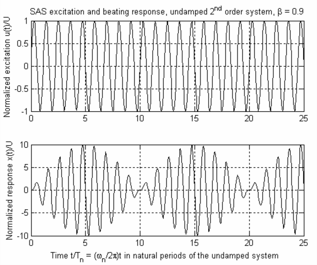
The apparent period of beating is the interval between successive minima or successive maxima of response, \(10 T_{n}\) in the case of Figure \(\PageIndex{1}\), which is half the period of the amplitude-modulating term. Therefore, the apparent frequency of beating is \(\left|\omega-\omega_{n}\right|\), which is twice the frequency of the amplitude-modulating term. Similarly, when we hear two musical tones of close but not identical pitches (frequencies), the frequency of beating that we perceive is the difference between the two tonal frequencies.

Let us consider now the remaining term, \(\left(1-\omega / \omega_{n}\right) \sin \omega_{n} t\), within the brackets of Equations \(\ref{eqn:10.40}\) and \(\ref{eqn:10.41}\). Pure undamped beating, in general, is the combination of two sinusoids that have different but closely spaced frequencies, as the two sinusoids pass into and out of phase with each other. The beating of the undamped 2^nd order system shown on Figure \(\PageIndex{1}\) is the combination of two sinusoids in the term \(\sin \omega t-\sin \omega_{n} t\) of Equation \(\ref{eqn:10.38}\). These two sinusoids represent

1. the driven response of the system at the excitation frequency \(\omega\), and
2. most of the free-vibration response of the system at its natural frequency \(\omega_{n}\).

When these two sinusoids are in phase, they combine and, together with the smaller contribution of the term \(\left(1-\omega / \omega_{n}\right) \sin \omega_{n} t\), form the maximal response; when they are out of phase, they nullify each other completely, leaving only the small remaining part of the free-vibration response due to the term \(\left(1-\omega / \omega_{n}\right) \sin \omega_{n} t\).

Thus far, we have examined response to suddenly applied sinusoidal excitation of a physically unrealistic undamped 2^nd order system. Let us consider next the influence of more realistic subcritical damping by solving for complete time response of an underdamped 2^nd order system the ODE \(\ddot{x}+2 \zeta \omega_{n} \dot{x}+\omega_{n}^{2} x=\omega_{n}^{2} u(t)\) with \(u(t) = 0\) for \(t < 0\) and \(u(t)=U \sin \omega t\) for \(t \geq 0\), and with rest ICs \(x(0)=0\) and \(\dot{x}(0)=0\). An appropriate convolution-integral solution is Equation 9.3.8:

\[x(t)=\frac{\omega_{n}^{2}}{\omega_{d}} \int_{\tau=0}^{\tau=t} e^{-\zeta \omega_{n} \tau} \sin \omega_{d} \tau \times u(t-\tau) d \tau=\frac{\omega_{n}^{2}}{\omega_{d}} \int_{\tau=0}^{\tau=t} e^{-\zeta \omega_{n} \tau} \sin \omega_{d} \tau \times U \sin \omega(t-\tau) d \tau \nonumber \]

The damped frequency is \(\omega_{d} \equiv \omega_{n} \sqrt{1-\zeta^{2}}\), so we can express the response integral in dimensionless form as

\[\frac{x(t)}{U}=\frac{\omega_{n}}{\sqrt{1-\zeta^{2}}} \int_{\tau=0}^{\tau=t} e^{-\zeta \omega_{n} \tau} \sin \omega_{n} \sqrt{1-\zeta^{2}} \tau \times \sin \omega(t-\tau) d \tau\label{eqn:10.42} \]

After evaluation of the formidable integral in Equation \(\ref{eqn:10.42}\), the solution is¹

\[\frac{x(t)}{U}=\frac{e^{-\zeta \omega_{n} t} \beta\left[2 \zeta \cos \omega_{d} t-\frac{\left(1-\beta^{2}-2 \zeta^{2}\right)}{\sqrt{1-\zeta^{2}}} \sin \omega_{d} t\right]+\left(1-\beta^{2}\right) \sin \omega t-2 \zeta \beta \cos \omega t}{\left(1-\beta^{2}\right)^{2}+(2 \zeta \beta)^{2}}\label{eqn:10.43} \]

The equation for response of an undamped 2^nd order system that is most similar in algebraic form to Equation \(\ref{eqn:10.43}\) is Equation \(\ref{eqn:10.37}\), and you can easily show that for \(\zeta=0\) Equation \(\ref{eqn:10.43}\) reduces to Equation \(\ref{eqn:10.37}\). However, unlike Equation \(\ref{eqn:10.37}\), Equation \(\ref{eqn:10.43}\) apparently cannot be reconfigured into a form comparable to Equation \(\ref{eqn:10.40}\) that is amenable to physical interpretation relative to beating behavior. To learn the physical character of Equation \(\ref{eqn:10.43}\), it seems that the best we can do is to evaluate it computationally with relevant numerical parameters and then interpret the results. For computation of Equation \(\ref{eqn:10.43}\), with definitions of driving frequency ratio \(\beta \equiv \omega / \omega_{n}\) and natural period \(T_{n} \equiv 2 \pi / \omega_{n}\), we can express the time-dependent function arguments of Equation \(\ref{eqn:10.43}\) in the following forms in terms of dimensionless time \(t / T_{n}\): \(-\zeta \omega_{n} t=-2 \pi \zeta\left(t / T_{n}\right), \omega_{d} t=2 \pi \sqrt{1-\zeta^{2}}\left(t / T_{n}\right)\), and \(\omega t=2 \pi \beta\left(t / T_{n}\right)\). Figure \(\PageIndex{2}\) includes plots of SAS response calculated from Equation \(\ref{eqn:10.43}\) for zero damping and for light viscous damping ratios \(\zeta\) = 0.01 and 0.02, with the excitation frequency set at 90% of the natural frequency, \(\omega=0.9 \omega_{n}\) or \(\beta=0.9\), the same as for Figure \(\PageIndex{1}\).

Figure \(\PageIndex{2}\): Calculations of Equation \(\ref{eqn:10.43}\) for a standard 2^nd order system having undamped natural frequency \(\omega_{n}\), with zero damping (top) and two positive values of viscous damping ratio, \(\zeta\) = 0.01 and 0.02; response from rest initial conditions to a suddenly applied (at \(t\) = 0) sinusoidal (SAS) excitation with frequency \(\omega=0.9 \omega_{n}\).

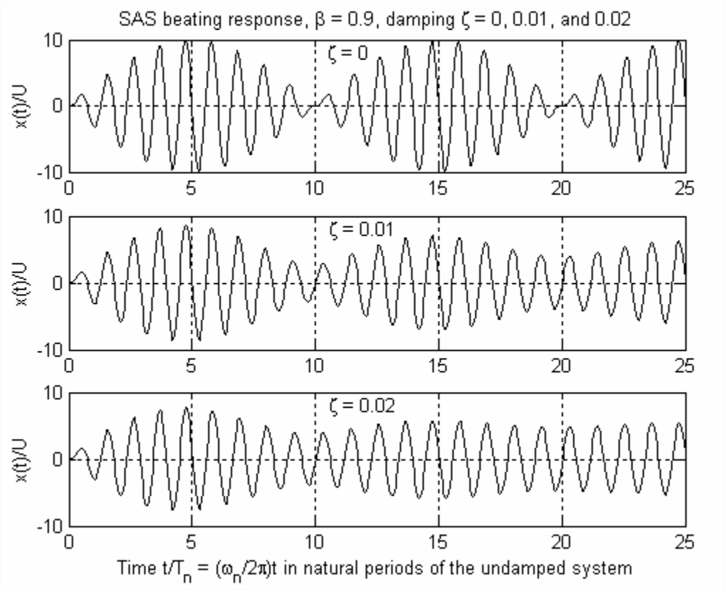
The response in Figure \(\PageIndex{2}\) for \(\zeta = 0\) is, of course, the same as that in Figure \(\PageIndex{1}\), with very significant beating. However, the responses for \(\zeta\) = 0.01 and 0.02 show that even these relatively small quantities of damping suppress the beating, at least for this case of \(\omega=0.9 \omega_{n}\). Although less obvious than for zero damping, the apparent period of beating for \(\zeta=0.01\), \(\sim 10 T_{n}\), is still quite evident. However, for \(\zeta=0.02\), the response in Figure \(\PageIndex{2}\) after 25 natural periods has almost settled into its steady-state condition, for which you can calculate from Equation 10.2.7 that the steady-state frequency-response magnitude ratio is \(X / U=5.171\). To investigate the nature of beating for any other case of damping ratio \(\zeta>0\) and excitation frequency ratio \(\beta \equiv \omega / \omega_{n}\), we would need again to evaluate Equation \(\ref{eqn:10.43}\) numerically; see, for example, homework Problem 10.17.

¹The author derived Equation \(\ref{eqn:10.43}\) first with MATLAB by applying the syms, int, simple, and pretty symbolic operations, and then by implementing the human touch with pencil and paper to simplify further the MATLAB result. See homework Problems 1.6 and 1.9.