14.2: Definitions and Examples of Open-Loop Control Systems

As an initial attempt to produce the desired motion history \(\theta(t)\), it is probably most natural simply to seek the input setting \(r(t)\) that will do the job completely, without the need for any further design refinement. This type of control is called open-loop control, for reasons that will be given later. Figure \(\PageIndex{1}\) depicts an open-loop control system.

Figure \(\PageIndex{1}\): Functional diagram of open-loop rotor-position control system. (Copyright; author via source)

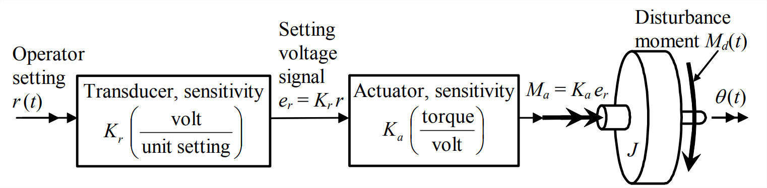
Operator setting \(r(t)\) is shown in Figure \(\PageIndex{1}\) as a general quantity, and the input transducer is assumed to be a general linear device that produces voltage signal \(e_{r}(t)=K_{r} r(t)\); if the input device were a rotary dial, for example, the operator setting might be a rotational position in degrees, and the transducer might be a variable resistor in a voltage divider circuit (see homework Problems 5.1 and 5.9), with accurately calibrated sensitivity of \(K_r\) volts per degree. The actuator also is assumed to be a general linear device that produces control moment \(M_{a}(t)=K_{a} e_{r}(t)=K_{a} K_{r} r(t)\); if it were an electromagnetic actuator, for example, it would probably consist of a power amplifier and a motor, both of which are designed to function linearly. In practice, device sensitivity constants do not have to be positive and often are negative, but let’s assume here that all are positive (\(K_a > 0\), \(K_r > 0\), etc.) just to avoid unnecessary complications.

Also shown on Figure \(\PageIndex{1}\) is disturbance moment \(M_{d}(t)\) acting upon the rotor. In the terminology of control, a disturbance is some extraneous action upon the plant, not the intended control action. In the system of Figure \(\PageIndex{1}\), for example, an actuator moment produced by unwanted electrical noise in the circuitry would be an internal disturbance, and a moment produced by wind or impact from solid objects onto the rotor would be an external disturbance. Disturbances are often random, or at least unpredictable, so that we usually cannot write equations to describe their variation with time. In most cases, disturbances tend to influence adversely the performance of a control system.

Let us analyze the control system of Figure \(\PageIndex{1}\). The total moment acting upon the rotor is \(M_{a}(t)+M_{d}(t)\), so that Equation 14.1.1 becomes

\[J \ddot{\theta}=M_{a}(t)+M_{d}(t)=K_{a} K_{r} r(t)+M_{d}(t)\label{eqn:14.4} \]

Disturbance \(M_{d}(t)\) in Equation \(\ref{eqn:14.4}\) is the nemesis of open-loop control, so let us consider initially the case with zero disturbance, \(M_{d}(t)=0\). If we have an equation for the desired motion history \(\theta(t)\), then we can solve Equation \(\ref{eqn:14.4}\) directly for the required operator setting:

\[r(t)=\frac{J}{K_{a} K_{r}} \ddot{\theta}\label{eqn:14.5} \]

This method for finding \(r(t)\) is easy, and open-loop control appears to be a feasible engineering tool. However, open-loop control has some serious deficiencies. A more detailed example will help to reveal these deficiencies, so we consider next an application of open-loop attitude control for a spacecraft.

Suppose that a capsule carrying astronauts is re-entering Earth’s atmosphere, Figure \(\PageIndex{2}\), and that pitch angle \(\theta(t)\) must be controlled in order to position the heat shield for optimal functioning and to prevent unstable tumbling. Two collinear pairs of gas thrusters (usually fueled by liquid chemicals) are separated by moment arm e so that they actuate rotation by a couple (pure moment), without causing mass center \(C\) to translate. Firing of the two thrusters shown active on Figure \(\PageIndex{2}\) produces a positive couple, and firing of the two opposite collinear thrusters would produce a negative couple. To simplify the analysis, let us assume that the thrusters are continuously throttleable, so that thrust force is related linearly to the operator setting by

\[f_{v}(t)=K r(t)\label{eqn:14.6} \]

Figure \(\PageIndex{2}\): Pitch control of a re-entry capsule. (Copyright; author via source)

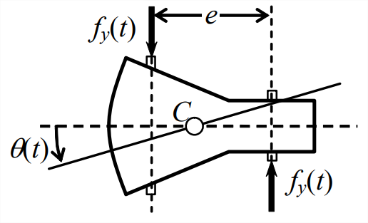
In Equation \(\ref{eqn:14.6}\), \(K\) is a positive sensitivity constant, with appropriate dimensions depending upon the specific character of \(r(t)\). Then the control moment is \(M_{a}(t)=e f_{y}(t)=e K r(t)\), so at the equation of motion equivalent to Equation \(\ref{eqn:14.4}\) is

\[J \ddot{\theta}=M_{a}(t)+M_{d}(t)=e K r(t)+M_{d}(t)\label{eqn:14.7} \]

in which J is the capsule’s rotational inertia about mass center \(C\). If we neglect all possible disturbances, \(M_{d}(t)=0\), then we can solve Equation \(\ref{eqn:14.7}\) for the required operator setting in terms of the desired pitching maneuver:

\[r(t)=\frac{J}{e K} \ddot{\theta}\label{eqn:14.8} \]

For example, let us require that the spacecraft rotate smoothly from \(\theta = 0\) to final pitch angle \(\theta=\theta_{f}\) during \(t_f\) seconds, according to the lower time history graphed on Figure \(\PageIndex{3}\), which is expressed by the equation¹

\[\theta(t)=\frac{\theta_{f}}{\pi}\left[\frac{\pi}{t_{f}} t-\frac{1}{2} \sin \left(\frac{2 \pi}{t_{f}} t\right)\right]\label{eqn:14.9} \]

for \(0 \leq t \leq t_{f}\). Differentiating Equation \(\ref{eqn:14.9}\) twice and then substituting the result into Equation \(\ref{eqn:14.8}\) leads to

\[r(t)=r_{A} \sin \left(\frac{2 \pi}{t_{f}} t\right), \quad r_{A} \equiv \frac{2 \pi J \theta_{f}}{e K t_{f}^{2}}, \quad \text { for } 0 \leq t \leq t_{f}\label{eqn:14.10} \]

This reference input setting \(r(t)\) is shown on the upper graph of Figure \(\PageIndex{3}\).

Figure \(\PageIndex{3}\): Example operator setting and resulting pitch maneuver for re-entry capsule. (Copyright; author via source)

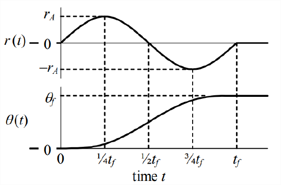
Note that Equations \(\ref{eqn:14.9}\) and \(\ref{eqn:14.10}\) and Figure \(\PageIndex{3}\) illustrate the impulse-momentum theorem for 1-DOF rotation, which is directly analogous to the impulse-momentum theorem for 1-DOF translation (Section 8.2). The control moment is proportional to \(r(t)\), \(M_{a}(t)=e K r(t)\), so the \(r(t)\) time history shows that the total moment impulse (area under the moment curve) in this maneuver is zero; since the total impulse is zero, the final (\(t \geq t_{f}\)) angular momentum also is zero, \(J \dot{\theta}=0\), so the spacecraft is rotated to the final position \(\theta=\theta_{f}\) with zero final rotational velocity, \(\dot{\theta}=0\).

Let us pause for a reality check. One feature of the control equipment described for this spacecraft maneuver is not practically realistic: space qualified gas thrusters in common use are nonlinear on-off (approximately) force generators; they are not continuously throttleable as assumed in this example, Equation \(\ref{eqn:14.6}\). Gas thrusters are, in fact, used to actuate spacecraft attitude and position control, but their on-off character produces rougher motion (abrupt changes in acceleration) than that of Equation \(\ref{eqn:14.9}\); see Sarafin, 1995, pp. 636-637. A smooth maneuver such as Equation \(\ref{eqn:14.9}\) would be actuated in practice by a space-qualified reaction wheel or control-moment gyroscope. We have assumed the hypothetical throttleable gas thrusters for this example just because it is easy to visualize this situation and to describe it in equations.

Now, with reference to the example above of spacecraft attitude control, let us evaluate open-loop control as represented generally by Figure \(\PageIndex{1}\), with particular interest in identifying the following deficiencies:

1. Note from Figure \(\PageIndex{3}\) that output \(\theta(t)\) is not a single-valued, monotonic function of operator setting \(r(t)\). For example, to \(r = 0\) there correspond three different output values: \(\theta = 0\) before the maneuver, \(\theta=1 / 2 \theta_{f}\) during the maneuver, and \(\theta=\theta_{f}\) after the maneuver. This type of complicated functional relationship is not necessarily an operational deficiency, but it certainly is counter-intuitive to the natural engineering expectation of a unique, monotonic, often linear relationship between cause and effect.
2. Equations \(\ref{eqn:14.5}\), \(\ref{eqn:14.8}\), and \(\ref{eqn:14.10}\) show that the validity of derived operator setting \(r(t)\) is directly dependent upon the accuracy of the plant parameters and control system sensitivities, and upon the fidelity of the theoretical model of the system. If, for example, we use an inaccurate value of rotational inertia \(J\) (a distinct possibility for most vehicles, since burning of fuel changes inertias), or if the thrusters fail to function exactly as we model them, then the derived \(r(t)\) clearly will not lead to the exact desired rotation time history, \(\theta(t)\).
3. The \(r(t)\) Equations \(\ref{eqn:14.5}\) and \(\ref{eqn:14.8}\) are predicated on the absence of disturbances; but if \(M_{d}(t) \neq 0\), then the derived \(r(t)\) will fail to produce the exact desired \(\theta(t)\). In practice, unpredictable disturbances are common, and they should not be ignored. For example, moments that can act upon a re-entering spacecraft might be produced by atmospheric drag, impact from space debris, astronauts shifting position within the vehicle, etc.

Deficiencies 2 and 3 above can be described in a more general manner: the performance of an open-loop control system is strongly dependent upon the quality of the theoretical model of the system and its environment; in other words, the control performance is highly sensitive to imperfections in the theoretical model, which are inevitable for most real engineering situations.²

It is a fundamental characteristic and weakness of open-loop control that the actual output is not measured and compared with the desired output, for the purposes of assessing the output error and attempting to reduce the error. A simple and natural remedy for this weakness is to “close the loop” with feedback, which is described in the next section. Note that the absence of a feedback branch from Figure \(\PageIndex{1}\) leads to the designation “open-loop.” But even this designation is at least a little misleading because there is no “loop” at all; there is simply a single branch that carries forward-flowing signals!

¹Maneuver time history Equation \(\ref{eqn:14.9}\) comes from Sarafin, 1995, pages 644-645, a book that includes additional interesting discussions of spacecraft attitude control.

²In the language of control engineering, a control system is described as robust if its performance and stability are insensitive to potentially detrimental influences such as disturbances, deficiencies in the theoretical model of the plant, and inaccurate response measurements due to sensor dynamics.