1.7: Discrete Time Impulse Function

Last updated
Save as PDF

Page ID: 23113

\( \newcommand{\vecs}[1]{\overset { \scriptstyle \rightharpoonup} {\mathbf{#1}} } \) \( \newcommand{\vecd}[1]{\overset{-\!-\!\rightharpoonup}{\vphantom{a}\smash {#1}}} \)\(\newcommand{\id}{\mathrm{id}}\) \( \newcommand{\Span}{\mathrm{span}}\) \( \newcommand{\kernel}{\mathrm{null}\,}\) \( \newcommand{\range}{\mathrm{range}\,}\) \( \newcommand{\RealPart}{\mathrm{Re}}\) \( \newcommand{\ImaginaryPart}{\mathrm{Im}}\) \( \newcommand{\Argument}{\mathrm{Arg}}\) \( \newcommand{\norm}[1]{\| #1 \|}\) \( \newcommand{\inner}[2]{\langle #1, #2 \rangle}\) \( \newcommand{\Span}{\mathrm{span}}\) \(\newcommand{\id}{\mathrm{id}}\) \( \newcommand{\Span}{\mathrm{span}}\) \( \newcommand{\kernel}{\mathrm{null}\,}\) \( \newcommand{\range}{\mathrm{range}\,}\) \( \newcommand{\RealPart}{\mathrm{Re}}\) \( \newcommand{\ImaginaryPart}{\mathrm{Im}}\) \( \newcommand{\Argument}{\mathrm{Arg}}\) \( \newcommand{\norm}[1]{\| #1 \|}\) \( \newcommand{\inner}[2]{\langle #1, #2 \rangle}\) \( \newcommand{\Span}{\mathrm{span}}\)\(\newcommand{\AA}{\unicode[.8,0]{x212B}}\)

Introduction

In engineering, we often deal with the idea of an action occurring at a point. Whether it be a force at a point in space or some other signal at a point in time, it becomes worth while to develop some way of quantitatively defining this. This leads us to the idea of a unit impulse, probably the second most important function, next to the complex exponential, in this systems and signals course.

Unit Sample Function

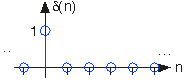
The unit sample function, often referred to as the unit impulse or delta function, is the function that defines the idea of a unit impulse in discrete time. There are not nearly as many intricacies involved in its definition as there are in the definition of the Dirac delta function, the continuous time impulse function. The unit sample function simply takes a value of one at \(n=0\) and a value of zero elsewhere. The impulse function is often written as \(\delta[n]\).

\[\delta[n]=\left\{\begin{array}{l}
1 \text { if } n=0 \\
0 \text { otherwise }
\end{array}\right. \nonumber \]

Figure \(\PageIndex{1}\): The unit sample.

Below we will briefly list a few important properties of the unit impulse without going into detail of their proofs.

Unit Impulse Properties

\(\delta[n]=\delta[-n]\)
\(\delta[n]=u[n]-u[n-1]\)
\(x[n] \delta[n]=x[0] \delta[n]\)

\[\sum_{n=-\infty}^{\infty} x[n] \delta[n]=\sum_{n=-\infty}^{\infty} x[0] \delta[n]=x[0] \sum_{n=-\infty}^{\infty} \delta[n]=x[0] \nonumber \]

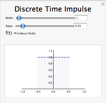
Discrete Time Impulse Response Demonstration

DTIDemo — Figure \(\PageIndex{2}\): Interact(when online) with a Mathematica CDF demonstrating the Discrete Time Impulse Function.

Discrete Time Unit Impulse Summary

The discrete time unit impulse function, also known as the unit sample function, is of great importance to the study of signals and systems. The function takes a value of one at time \(n=0\) and a value of zero elsewhere. It has several important properties that will appear again when studying systems.