9.5: Discrete Time Convolution and the DTFT

Last updated
Save as PDF

Page ID: 22897

\( \newcommand{\vecs}[1]{\overset { \scriptstyle \rightharpoonup} {\mathbf{#1}} } \) \( \newcommand{\vecd}[1]{\overset{-\!-\!\rightharpoonup}{\vphantom{a}\smash {#1}}} \)\(\newcommand{\id}{\mathrm{id}}\) \( \newcommand{\Span}{\mathrm{span}}\) \( \newcommand{\kernel}{\mathrm{null}\,}\) \( \newcommand{\range}{\mathrm{range}\,}\) \( \newcommand{\RealPart}{\mathrm{Re}}\) \( \newcommand{\ImaginaryPart}{\mathrm{Im}}\) \( \newcommand{\Argument}{\mathrm{Arg}}\) \( \newcommand{\norm}[1]{\| #1 \|}\) \( \newcommand{\inner}[2]{\langle #1, #2 \rangle}\) \( \newcommand{\Span}{\mathrm{span}}\) \(\newcommand{\id}{\mathrm{id}}\) \( \newcommand{\Span}{\mathrm{span}}\) \( \newcommand{\kernel}{\mathrm{null}\,}\) \( \newcommand{\range}{\mathrm{range}\,}\) \( \newcommand{\RealPart}{\mathrm{Re}}\) \( \newcommand{\ImaginaryPart}{\mathrm{Im}}\) \( \newcommand{\Argument}{\mathrm{Arg}}\) \( \newcommand{\norm}[1]{\| #1 \|}\) \( \newcommand{\inner}[2]{\langle #1, #2 \rangle}\) \( \newcommand{\Span}{\mathrm{span}}\)\(\newcommand{\AA}{\unicode[.8,0]{x212B}}\)

Introduction

This module discusses convolution of discrete signals in the time and frequency domains.

The Discrete-Time Convolution

Discrete Time Fourier Transform

The DTFT transforms an infinite-length discrete signal in the time domain into an finite-length (or \(2 \pi\)-periodic) continuous signal in the frequency domain.

DTFT

\[X(\omega)=\sum_{n=-\infty}^{\infty} x(n) e^{-(j \omega n)} \nonumber \]

Inverse DTFT

\[x(n)=\frac{1}{2 \pi} \int_{0}^{2 \pi} X(\omega) e^{j \omega n} d \omega \nonumber \]

Demonstration

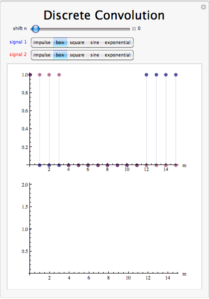
DiscreteConvolutionDemo — Figure \(\PageIndex{1}\): Interact (when online) with a Mathematica CDF demonstrating the Discrete Convolution. To Download, right-click and save as .cdf.

Convolution Sum

As mentioned above, the convolution sum provides a concise, mathematical way to express the output of an LTI system based on an arbitrary discrete-time input signal and the system's impulse response. The convolution sum is expressed as

\[y[n]=\sum_{k=-\infty}^{\infty} x[k] h[n-k] \nonumber \]

As with continuous-time, convolution is represented by the symbol \(*\), and can be written as

\[y[n]=x[n] * h[n] \nonumber \]

Convolution is commutative. For more information on the characteristics of convolution, read about the Properties of Convolution (Section 3.4).

Convolution Theorem

Let \(f\) and \(g\) be two functions with convolution \(f*g\). Let \(F\) be the Fourier transform operator. Then

\[F(f * g)=F(f) \cdot F(g) \nonumber \]

\[F(f \cdot g)=F(f) * F(g) \nonumber \]

By applying the inverse Fourier transform \(F^{−1}\), we can write:

\[f * g=F^{-1}(F(f) \cdot F(g)) \nonumber \]

Conclusion

The Fourier transform of a convolution is the pointwise product of Fourier transforms. In other words, convolution in one domain (e.g., time domain) corresponds to point-wise multiplication in the other domain (e.g., frequency domain).