4.3: Production Decline for Shale Gas Wells

Production Decline for Shale Gas Wells

Part of the reason for the rapid emergence of shale gas in the North American natural gas market has to do not only with the sheer number of wells drilled but also the production profile for shale gas wells over time. This production profile is referred to as the decline curve. The production profile of typical shale wells entails a rather sharp initial decline in the production rate and, after a few years, a much slower rate of decline. This becomes very important in determining the profitability of shale gas wells versus conventional gas wells. We'll return to this issue in the second half of the course. For now, we'll focus on being able to model the production profile of a shale gas well.

Illustrations of shale gas production decline curves are depicted below in \(Figure 4.1\), for two cases – one with 3.6 billion cubic feet of estimated ultimate recoverable reserves (EUR) and a second with 4.6 billion cubic feet EUR. Production in the initial several years of the well’s productive life declines hyperbolically, and at some point, the production decline levels off reflecting an exponential (constant annual percentage) decline rate.

The equation for hyperbolic decline, assuming that production decline is tracked monthly, is: \[P t=I P \times \frac{1}{(1+b \times D \times t)^{1 / b}}\]

where \(P_{t}\) is production during month \(t\), \(IP\) is the initial production rate (in million cubic feet per day), and \(b\) and \(D\) are parameters that are estimated based on the behavior of a particular well or similar wells.

Meanwhile, the equation for exponential decline is: \[P_{t}=I P \times e^{-D_{s} t}\]

where all variables are identical to those defined in equation (1), with the exception of \(D_{s}\), which is the monthly decline rate at the point where production shifts from hyperbolic to exponential tail decline.

As an example, suppose that initial production was 10 million cubic feet per day, and the value of the \(b\) and \(D\) parameters are 1.8 and 0.58, respectively. The well exhibits hyperbolic decline for the first 60 months and then shifts to exponential decline for the remainder of the well’s life.

We would thus estimate production in month 24 (i.e., at the end of the second year of production) as \(P_{24}=10 \times \frac{1}{(1+1.8 \times 0.58 \times 24)^{1 / 1.8}}=1.63\) million cubic feet per day.

As a second example (and a check that you understand how to use the formula), show for yourself that the production for this same well in month 47 would be 1.137 million cubic feet per day.

To estimate production at month 100 (past the transition point to exponential decline), we would take the production at the very end of the hyperbolic decline period (equal to 0.996 million cubic feet per day, which you should check yourself using the formula, using \(t = 60\)) as the initial production for exponential decline, and start counting time periods from that point. The decline parameter \(D_{s}\) for the exponential tail decline would be estimated as the percentage decline at the point where production shifts from hyperbolic to exponential.

We'll walk through this in a couple of steps. We have already calculated that production in month 60 is 0.996 million cubic feet per day. Assuming a continuation of hyperbolic decline, we would find that production in month 61 was 0.987 million cubic feet per day (again, check this yourself).

What we'll use for the decline parameter \(D_{s}\) in the exponential decline is the percentage difference between production in month 60 and month 61. So what we get for the exponential decline parameter is: \(D_{s}=(0.996-0.988) / 0.996=0.009\) (try it yourself).

From month 61 onwards, we would use the exponential decline function to estimate monthly production, with the month 60 production (0.996 million cubic feet per day) as the initial production and \({D}_{s}=0.009\) as the decline parameter. Moreover, we would start counting periods (the \(t\) variable in the exponential decline equation) from the transition point to exponential decline and not from the original initial production level of 10 million cubic feet per day.

Now, back to the question of production in month 100, which would be the 40th month of exponential decline. We use the exponential decline equation with \(IP = 0.996\) million cubic feet, \(t = 40\) months and \(D_{s} = 0.009\). Production in month 100 would be calculated as: \(P_{100}=0.996 \times e^{-0.009 \times 40}=0.695\) million cubic feet per day.

As another example for you to check your understanding, show that production in month 83 for this well would be estimated at 0.8098 million cubic feet per day.

Referring again to \(Figure \text { } 4.1\), average annual production from this hypothetical shale gas well is over 650 million cubic feet during the first year, about 300 million cubic feet during the second, after 8 years about 130 million cubic feet, and roughly 40 million cubic feet per year after 30 years of production. Note that these numbers are per-year production figures, not cumulative production figures over the life of the well.

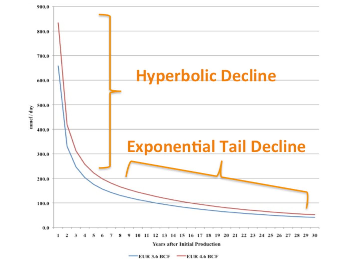
\(Figure \text { } 4.1\): Illustrative production decline curves for shale gas wells.

These decline curves are not just academic exercises. This sort of analysis is utilized to help determine whether specific shale energy development porjects are likely to pay off. The high initial production rate and steep initial decline is characteristic of shale wells (and is a lot different than the slower decline in many conventional gas wells), meaning that most of a project's revenues - sometimes as high as 80% of total lifetime well revenues - can accrued over the first five to seven years of the well's producing life. As we will see later in the course when we go through examples of financial analysis for a gas well project, the "front-loading" of production in shale wells can make a big difference in project economics.